I was so glad to be involved with this project of Hannah Hoffman. She had inquired on Twitter whether mathematicians could provide a proof of the irrationality of root two that rhymes. I set off immediately, of course, to answer the challenge. My wife Barbara Gail Montero and our daughter Hypatia and I spent a day thinking, writing, revising, rewriting, rethinking, rewriting, and eventually we had a set lyrics providing the proof, in rhyme and meter. We had wanted specifically to highlight not only the logic of the proof, but also to tell the fateful story of Hippasus, credited with the discovery.
Hannah proceeded to create the amazing musical version:
The diagonal of a square is incommensurable with its side
an astounding fact the Pythagoreans did hide
but Hippasus rebelled and spoke the truth
making his point with irrefutable proof
it’s absurd to suppose that the root of two
is rational, namely, p over q
square both sides and you will see
that twice q squared is the square of p
since p squared is even, then p is as well
now, if p as 2k you alternately spell
2q squared will to 4k squared equate
revealing, when halved, q’s even fate
thus, root two as fraction, p over q
must have numerator and denomerator with factors of two
to lowest terms, therefore, it can’t be reduced
root two is irrational, Hippasus deduced
as retribution for revealing this irrationality
Hippasus, it is said, was drowned in the sea
but his proof live on for the whole world to admire
a truth of elegance that will ever inspire.
This brief unpublished note (11 pages) contains an overview of the Gödel fixed-point lemma, along with several generalizations and applications, written for use in the Week 3 lecture of the Graduate Philosophy of Logic seminar that I co-taught with Volker Halbach at Oxford in Hilary term 2021. The theme of the seminar was self-reference, truth, and consistency strengths, and in this lecture we discussed the nature of Gödel’s fixed-point lemma and generalizations, with various applications in logic.
Gödel’s fixed-point lemma An application to the Gödel incompleteness theorem
Finite self-referential schemes An application to nonindependent disjunctions of independent sentences
Gödel-Carnap fixed point lemma Deriving the double fixed-point lemma as a consequence An application to the provability version of Yablo’s paradox
Kleene recursion theorem An application involving computable numbers An application involving the universal algorithm An application to Quine programs and Ouroborous chains
Welcome to Cantor’s Ice Cream Shoppe! A huge choice of flavors—pile your cone high with as many scoops as you want!
Have two scoops, or three, four, or more! Why not infinitely many? Would you like $\omega$ many scoops, or $\omega\cdot2+5$ many scoops? You can have any countable ordinal number of scoops on your cone.
And furthermore, after ordering your scoops, you can order more scoops to be placed on top—all I ask is that you let me know how many such extra orders you plan to make. Let’s simply proceed transfinitely. You can announce any countable ordinal $\eta$, which will be the number of successive orders you will make; each order is a countable ordinal number of ice cream scoops to be placed on top of whatever cone is being assembled.
In fact, I’ll even let you change your mind about $\eta$ as we proceed, so as to give you more orders to make a taller cone.
So the process is:
You pick a countable ordinal $\eta$, which is the number of orders you will make.
For each order, you can pick any countable ordinal number of scoops to be added to the top of your ice-cream cone.
After making your order, you can freely increase $\eta$ to any larger countable ordinal, giving you the chance to make as many additional orders as you like.
At each limit stage of the ordering process, the ice cream cone you are assembling has all the scoops you’ve ordered so far, and we set the current $\eta$ value to the supremum of the values you had chosen so far.
If at any stage, you’ve used up your $\eta$ many orders, then the process has completed, and I serve you your ice cream cone. Enjoy!
Question. Can you arrange to achieve uncountably many scoops on your cone?
Although at each stage we place only countably many ice cream scoops onto the cone, nevertheless we can keep giving ourselves extra stages, as many as we want, simply by increasing $\eta$. Can you describe a systematic process of increasing the number of steps that will enable you to make uncountably many orders? This would achieve an unountable ice cream cone.
What is your solution? Give it some thought before proceeding. My solution appears below.
Alas, I claim that at Cantor’s Ice Cream Shoppe you cannot make an ice cream cone with uncountably many scoops. Specifically, I claim that there will inevitably come a countable ordinal stage at which you have used up all your orders.
Suppose that you begin by ordering $\beta_0$ many scoops, and setting a large value $\eta_0$ for the number of orders you will make. You subsequently order $\beta_1$ many additional scoops, and then $\beta_2$ many on top of that, and so on. At each stage, you may also have increased the value of $\eta_0$ to $\eta_1$ and then $\eta_2$ and so on. Probably all of these are enormous countable ordinals, making a huge ice cream cone.
At each stage $\alpha$, provided $\alpha<\eta_\alpha$, then you can make an order of $\beta_\alpha$ many scoops on top of your cone, and increase $\eta_\alpha$ to $\eta_{\alpha+1}$, if desired, or keep it the same.
At a limit stage $\lambda$, your cone has $\sum_{\alpha<\lambda}\beta_\alpha$ many scoops, and we update the $\eta$ value to the supremum of your earlier declarations $\eta_\lambda=\sup_{\alpha<\lambda}\eta_\alpha$.
What I claim now is that there will inevitably come a countable stage $\lambda$ for which $\lambda=\eta_\lambda$, meaning that you have used up all your orders with no possibility to further increase $\eta$. To see this, consider the sequence $$\eta_0\leq \eta_{\eta_0}\leq \eta_{\eta_{\eta_0}}\leq\cdots$$ We can define the sequence recursively by $\lambda_0=\eta_0$ and $\lambda_{n+1}=\eta_{\lambda_n}$. Let $\lambda=\sup_{n<\omega}\lambda_n$, the limit of this sequence. This is a countable supremum of countable ordinals and hence countable. But notice that $$\eta_\lambda=\sup_{n<\omega}\eta_{\lambda_n}=\sup_{n<\omega}\lambda_{n+1}=\lambda.$$ That is, $\eta_\lambda=\lambda$ itself, and so your orders have run out at $\lambda$, with no possibility to add more scoops or to increase $\eta$. So your order process completed at a countable stage, and you have therefore altogether only a countable ordinal number of scoops of ice cream. I’m truly very sorry at your pitiable impoverishment.
I’d like to introduce and discuss the otherworldly cardinals, a large cardinal notion that frequently arises in set-theoretic analysis, but which until now doesn’t seem yet to have been given its own special name. So let us do so here.
I was put on to the topic by Jason Chen, a PhD student at UC Irvine working with Toby Meadows, who brought up the topic recently on Twitter:
Do these cardinals have special names: α's such that there is some β with V_α being an elementary substructure of V_β (so they form a proper subset of worldly cardinals); and a stratified version: α's such that there is some β, with V_α being a Σ_n-elementary substructure of V_β.
In response, I had suggested the otherworldly terminology, a play on the fact that the two cardinals will both be worldly, and so we have in essence two closely related worlds, looking alike. We discussed the best way to implement the terminology and its extensions. The main idea is the following:
Main Definition. An ordinal $\kappa$ is otherworldly if $V_\kappa\prec V_\lambda$ for some ordinal $\lambda>\kappa$. In this case, we say that $\kappa$ is otherworldly to $\lambda$.
It is an interesting exercise to see that every otherworldly cardinal $\kappa$ is in fact also worldly, which means $V_\kappa\models\text{ZFC}$, and from this it follows that $\kappa$ is a strong limit cardinal and indeed a $\beth$-fixed point and even a $\beth$-hyperfixed point and more.
Theorem. Every otherworldly cardinal is also worldly.
Proof. Suppose that $\kappa$ is otherworldly, so that $V_\kappa\prec V_\lambda$ for some ordinal $\lambda>\kappa$. It follows that $\kappa$ must in fact be a cardinal, since otherwise it would be the order type of a relation on a set in $V_\kappa$, which would be isomorphic to an ordinal in $V_\lambda$ but not in $V_\kappa$. And since $\omega$ is not otherworldly, we see that $\kappa$ must be an uncountable cardinal. Since $V_\kappa$ is transitive, we get now easily that $V_\kappa$ satisfies extensionality, regularity, union, pairing, power set, separation and infinity. The only axiom remaining is replacement. If $\varphi(a,b)$ obeys a functional relation in $V_\kappa$ for all $a\in A$, where $A\in V_\kappa$, then $V_\lambda$ agrees with that, and also sees that the range is contained in $V_\kappa$, which is a set in $V_\lambda$. So $V_\kappa$ agrees that the range is a set. So $V_\kappa$ fulfills the replacement axiom. $\Box$
Corollary. A cardinal is otherworldly if and only if it is fully correct in a worldly cardinal.
Proof. Once you know that otherworldly cardinals are worldly, this amounts to a restatement of the definition. If $V_\kappa\prec V_\lambda$, then $\lambda$ is worldly, and $V_\kappa$ is correct in $V_\lambda$. $\Box$
Let me prove next that whenever you have an otherworldly cardinal, then you will also have a lot of worldly cardinals, not just these two.
Theorem. Every otherworldly cardinal $\kappa$ is a limit of worldly cardinals. What is more, every otherworldly cardinal is a limit of worldly cardinals having exactly the same first-order theory as $V_\kappa$, and indeed, the same $\alpha$-order theory for any particular $\alpha<\kappa$.
Proof. If $V_\kappa\prec V_\lambda$, then $V_\lambda$ can see that $\kappa$ is worldly and has the theory $T$ that it does. So $V_\lambda$ thinks, about $T$, that there is a cardinal whose rank initial segment has theory $T$. Thus, $V_\kappa$ also thinks this. And we can find arbitrarily large $\delta$ up to $\kappa$ such that $V_\delta$ has this same theory. This argument works whether one uses the first-order theory, or the second-order theory or indeed the $\alpha$-order theory for any $\alpha<\kappa$. $\Box$
Theorem. If $\kappa$ is otherworldly, then for every ordinal $\alpha<\kappa$ and natural number $n$, there is a cardinal $\delta<\kappa$ with $V_\delta\prec_{\Sigma_n}V_\kappa$ and the $\alpha$-order theory of $V_\delta$ is the same as $V_\kappa$.
Proof. One can do the same as above, since $V_\lambda$ can see that $V_\kappa$ has the $\alpha$-order theory that it does, while also agreeing on $\Sigma_n$ truth with $V_\lambda$, so $V_\kappa$ will agree that there should be such a cardinal $\delta<\kappa$. $\Box$
Definition. We say that a cardinal is totally otherworldly, if it is otherworldly to arbitrarily large ordinals. It is otherworldly beyond $\theta$, if it is otherworldly to some ordinal larger than $\theta$. It is otherworldly up to $\delta$, if it is otherworldly to ordinals cofinal in $\delta$.
Theorem. Every inaccessible cardinal $\delta$ is a limit of otherworldly cardinals that are each otherworldly up to and to $\delta$.
Proof. If $\delta$ is inaccessible, then a simple Löwenheim-Skolem construction shows that $V_\kappa$ is the union of a continuous elementary chain $$V_{\kappa_0}\prec V_{\kappa_1}\prec\cdots\prec V_{\kappa_\alpha}\prec \cdots \prec V_\kappa$$ Each of the cardinals $\kappa_\alpha$ arising on this chain is otherworldly up to and to $\delta$. $\Box$
Theorem. Every totally otherworldly cardinal is $\Sigma_2$ correct, meaning $V_\kappa\prec_{\Sigma_2} V$. Consequently, every totally otherworldly cardinal is larger than the least measurable cardinal, if it exists, and larger than the least superstrong cardinal, if it exists, and larger than the least huge cardinal, if it exists.
Proof. Every $\Sigma_2$ assertion is locally verifiable in the $V_\alpha$ hierarchy, in that it is equivalent to an assertion of the form $\exists\eta V_\eta\models\psi$ (for more information, see my post about Local properties in set theory). Thus, every true $\Sigma_2$ assertion is revealed inside any sufficiently large $V_\lambda$, and so if $V_\kappa\prec V_\lambda$ for arbitrarily large $\lambda$, then $V_\kappa$ will agree on those truths. $\Box$
I was a little confused at first about how two totally otherwordly cardinals interact, but now everything is clear with this next result. (Thanks to Hanul Jeon for his helpful comment below.)
Theorem. If $\kappa<\delta$ are both totally otherworldly, then $\kappa$ is otherworldly up to $\delta$, and hence totally otherworldly in $V_\delta$.
Proof. Since $\delta$ is totally otherworldly, it is $\Sigma_2$ correct. Since for every $\alpha<\delta$ the cardinal $\kappa$ is otherworldly beyond $\alpha$, meaning $V_\kappa\prec V_\lambda$ for some $\lambda>\alpha$, then since this is a $\Sigma_2$ feature of $\kappa$, it must already be true inside $V_\delta$. So such a $\lambda$ can be found below $\delta$, and so $\kappa$ is otherworldly up to $\delta$. $\Box$
Theorem. If $\kappa$ is totally otherworldly, then $\kappa$ is a limit of otherworldly cardinals, and indeed, a limit of otherworldly cardinals having the same theory as $V_\kappa$.
Proof. Assume $\kappa$ is totally otherworldly, let $T$ be the theory of $V_\kappa$, and consider any $\alpha<\kappa$. Since there is an otherworldly cardinal above $\alpha$ with theory $T$, namely $\kappa$, and because this is a $\Sigma_2$ fact about $\alpha$ and $T$, it follows that there must be such a cardinal above $\alpha$ inside $V_\kappa$. So $\kappa$ is a limit of otherworldly cardinals with the same theory as $V_\kappa$. $\Box$
The results above show that the consistency strength of the hypotheses are ordered as follows, with strict increases in consistency strength as you go up (assuming consistency):
ZFC + there is an inaccessible cardinal
ZFC + there is a proper class of totally otherworldly cardinals
ZFC + there is a totally otherworldly cardinal
ZFC + there is a proper class of otherworldly cardinals
ZFC + there is an otherworldly cardinal
ZFC + there is a proper class of worldly cardinals
ZFC + there is a worldly cardinal
ZFC + there is a transitive model of ZFC
ZFC + Con(ZFC)
ZFC
We might consider the natural strengthenings of otherworldliness, where one wants $V_\kappa\prec V_\lambda$ where $\lambda$ is itself otherworldly. That is, $\kappa$ is the beginning of an elementary chain of three models, not just two. This is different from having merely that $V_\kappa\prec V_\lambda$ and $V_\kappa\prec V_\eta$ for some $\eta>\lambda$, because perhaps $V_\lambda$ is not elementary in $V_\eta$, even though $V_\kappa$ is. Extending successively is a more demanding requirement.
One then naturally wants longer and longer chains, and ultimately we find ourselves considering various notions of rank in the rank elementary forest, which is the relation $\kappa\preceq\lambda\iff V_\kappa\prec V_\lambda$. The otherworldly cardinals are simply the non-maximal nodes in this order, while it will be interesting to consider the nodes that can be extended to longer elementary chains.
Consider the real numbers $\newcommand\R{\mathbb{R}}\R$ and the complex numbers $\newcommand\C{\mathbb{C}}\C$ and the question of whether these structures are interpretable in one another as fields.
What does it mean to interpret one mathematical structure in another? It means to provide a definable copy of the first structure in the second, by providing a definable domain of $k$-tuples (not necessarily just a domain of points) and definable interpretations of the atomic operations and relations, as well as a definable equivalence relation, a congruence with respect to the operations and relations, such that the first structure is isomorphic to the quotient of this definable structure by that equivalent relation. All these definitions should be expressible in the language of the host structure.
One may proceed recursively to translate any assertion in the language of the interpreted structure into the language of the host structure, thereby enabling a complete discussion of the first structure purely in the language of the second.
For an example, we can define a copy of the integer ring $\langle\mathbb{Z},+,\cdot\rangle$ inside the semi-ring of natural numbers $\langle\mathbb{N},+,\cdot\rangle$ by considering every integer as the equivalence class of a pair of natural numbers $(n,m)$ under the same-difference relation, by which $$(n,m)\equiv(u,v)\iff n-m=u-v\iff n+v=u+m.$$ Integer addition and multiplication can be defined on these pairs, well-defined with respect to same difference, and so we have interpreted the integers in the natural numbers.
Similarly, the rational field $\newcommand\Q{\mathbb{Q}}\Q$ can be interpreted in the integers as the quotient field, whose elements can be thought of as integer pairs $(p,q)$ written more conveniently as fractions $\frac pq$, where $q\neq 0$, considered under the same-ratio relation $$\frac pq\equiv\frac rs\qquad\iff\qquad ps=rq.$$ The field structure is now easy to define on these pairs by the familiar fractional arithmetic, which is well-defined with respect to that equivalence. Thus, we have provided a definable copy of the rational numbers inside the integers, an interpretation of $\Q$ in $\newcommand\Z{\mathbb{Z}}\Z$.
The complex field $\C$ is of course interpretable in the real field $\R$ by considering the complex number $a+bi$ as represented by the real number pair $(a,b)$, and defining the operations on these pairs in a way that obeys the expected complex arithmetic.
$$(a,b)+(c,d) =(a+c,b+d)$$
$$(a,b)\cdot(c,d)=(ac-bd,ad+bc)$$
Thus, we interpret the complex number field $\C$ inside the real field $\R$.
Question. What about an interpretation in the converse direction? Can we interpret $\R$ in $\C$?
Although of course the real numbers can be viewed as a subfield of the complex numbers $$\R\subset\C,$$this by itself doesn’t constitute an interpretation, unless the submodel is definable. And in fact, $\R$ is not a definable subset of $\C$. There is no purely field-theoretic property $\varphi(x)$, expressible in the language of fields, that holds in $\C$ of all and only the real numbers $x$. But more: not only is $\R$ not definable in $\C$ as a subfield, we cannot even define a copy of $\R$ in $\C$ in the language of fields. We cannot interpret $\R$ in $\C$ in the language of fields.
Theorem. As fields, the real numbers $\R$ are not interpretable in the complex numbers $\C$.
We can of course interpret the real numbers $\R$ in a structure slightly expanding $\C$ beyond its field structure. For example, if we consider not merely $\langle\C,+,\cdot\rangle$ but add the conjugation operation $\langle\C,+,\cdot,z\mapsto\bar z\rangle$, then we can identify the reals as the fixed-points of conjugation $z=\bar z$. Or if we add the real-part or imaginary-part operators, making the coordinate structure of the complex plane available, then we can of course define the real numbers in $\C$ as those complex numbers with no imaginary part. The point of the theorem is that in the pure language of fields, we cannot define the real subfield nor can we even define a copy of the real numbers in $\C$ as any kind of definable quotient structure.
The theorem is well-known to model theorists, a standard observation, and model theorists often like to prove it using some sophisticated methods, such as stability theory. The main issue from that point of view is that the order in the real numbers is definable from the real field structure, but the theory of algebraically closed fields is too stable to allow it to define an order like that.
But I would like to give a comparatively elementary proof of the theorem, which doesn’t require knowledge of stability theory. After a conversation this past weekend with Jonathan Pila, Boris Zilber and Alex Wilkie over lunch and coffee breaks at the Robin Gandy conference, here is such an elementary proof, based only on knowledge concerning the enormous number of automorphisms of $\C$, a consequence of the categoricity of the complex field, which itself follows from the fact that algebraically closed fields of a given characteristic are determined by their transcedence degree over their prime subfield. It follows that any two transcendental elements of $\C$ are automorphic images of one another, and indeed, for any element $z\in\C$ any two complex numbers transcendental over $\Q(z)$ are automorphic in $\C$ by an automorphism fixing $z$.
Proof of the theorem. Suppose that we could interpret the real field $\R$ inside the complex field $\C$. So we would define a domain of $k$-tuples $R\subseteq\C^k$ with an equivalence relation $\simeq$ on it, and operations of addition and multiplication on the equivalence classes, such that the real field was isomorphic to the resulting quotient structure $R/\simeq$. There is absolutely no requirement that this structure is a submodel of $\C$ in any sense, although that would of course be allowed if possible. The $+$ and $\times$ of the definable copy of $\R$ in $\C$ might be totally strange new operations defined on those equivalence classes. The definitions altogether may involve finitely many parameters $\vec p=(p_1,\ldots,p_n)$, which we now fix.
As we mentioned, the complex number field $\C$ has an enormous number of automorphisms, and indeed, any two $k$-tuples $\vec x$ and $\vec y$ that exhibit the same algebraic equations over $\Q(\vec p)$ will be automorphic by an automorphism fixing $\vec p$. In particular, this means that there are only countably many isomorphism orbits of the $k$-tuples of $\C$. Since there are uncountably many real numbers, this means that there must be two $\simeq$-inequivalent $k$-tuples in the domain $R$ that are automorphic images in $\C$, by an automorphism $\pi:\C\to\C$ fixing the parameters $\vec p$. Since $\pi$ fixes the parameters of the definition, it will take $R$ to $R$ and it will respect the equivalence relation and the definition of the addition and multiplication on $R/\simeq$. Therefore, $\pi$ will induce an automorphism of the real field $\R$, which will be nontrivial precisely because $\pi$ took an element of one $\simeq$-equivalence class to another.
The proof is now completed by the observation that the real field $\langle\R,+,\cdot\rangle$ is rigid; it has no nontrivial automorphisms. This is because the order is definable (the positive numbers are precisely the nonzero squares) and the individual rational numbers must be fixed by any automorphism and then every real number is determined by its cut in the rationals. So there can be no nontrivial automorphism of $\R$, and we have a contradiction. So $\R$ is not interpretable in $\C$. $\Box$
Let me introduce to you the topic of modal model theory, injecting some ideas from modal logic into the traditional subject of model theory in mathematical logic.
For example, we may consider the class of all models of some first-order theory, such as the class of all graphs, or the class of all groups, or all fields or what have you. In general, we have $\newcommand\Mod{\text{Mod}}\Mod(T)$, where $T$ is a first-order theory in some language $L$.
We may consider $\Mod(T)$ as a potentialist system, a Kripke model of possible worlds, where each model accesses the larger models, of which it is a submodel. So $\newcommand\possible{\Diamond}\possible\varphi$ is true at a model $M$, if there is a larger model $N$ in which $\varphi$ holds, and $\newcommand\necessary{\Box}\necessary\varphi$ is true at $M$, if $\varphi$ holds in all larger models.
In this way, we enlarge the language $L$ to include these modal operators. Let $\possible(L)$ be the language obtained by closing $L$ under the modal operators and Boolean connectives; and let $L^\possible$ also close under quantification. The difference is whether a modal operator falls under the scope of a quantifier.
Recently, in a collaborative project with Wojciech Aleksander Wołoszyn, we made some progress, which I’d like to explain. (We also have many further results, concerning the potentialist validities of various natural instances of $\Mod(T)$, but those will wait for another post.)
Theorem. If models $M$ and $N$ are elementarily equivalent, that is, if they have the same theory in the language of $L$, then they also have the same theory in the modal language $\possible(L)$.
Proof. We show that whenever $M\equiv N$ in the language of $L$, then $M\models\varphi\iff N\models\varphi$ for sentences $\varphi$ in the modal language $\possible(L)$, by induction on $\varphi$.
Of course, by assumption the statement is true for sentences $\varphi$ in the base language $L$. And the property is clearly preserved by Boolean combinations. What remains is the modal case. Suppose that $M\equiv N$ and $M\models\possible\varphi$. So there is some extension model $M\subset W\models\varphi$.
Since $M\equiv N$, it follows by the Keisler-Shelah theorem that $M$ and $N$ have isomorphic ultrapowers $\prod_\mu M\cong\prod_\mu N$, for some ultrafilter $\mu$. It is easy to see that isomorphic structures satisfy exactly the same modal assertions in the class of all models of a theory. Since $M\subset W$, it follows that the ultrapower of $M$ is extended to (a copy of) the ultrapower of $W$, and so $\prod_\mu M\models\possible\varphi$, and therefore also $\prod_\mu N\models\possible\varphi$. From this, since $N$ embeds into its ultrapower $\prod_\mu N$, it follows also that $N\models\possible\varphi$, as desired. $\Box$
Corollary. If one model elementarily embeds into another $M\prec N$, in the language $L$ of these structures, then this embedding is also elementary in the language $\possible(L)$.
Proof. To say $M\prec N$ in language $L$ is the same as saying that $M\equiv N$ in the language $L_M$, where we have added constants for every element of $M$, and interpreted these constants in $N$ via the embedding. Thus, by the theorem, it follows that $M\equiv N$ in the language $\possible(L_M)$, as desired. $\Box$
For example, every model $M$ is elementarily embedding into its ultrapowers $\prod_\mu M$, in the language $\possible(L)$.
We’d like to point out next that these results do not extend to elementary equivalence in the full modal language $L^\possible$.
For a counterexample, let’s work in the class of all simple graphs, in the language with a binary predicate for the edge relation. (We’ll have no parallel edges, and no self-edges.) So the accessibility relation here is the induced subgraph relation.
Lemma. The 2-colorability of a graph is expressible in $\possible(L)$. Similarly for $k$-colorability for any finite $k$.
Proof. A graph is 2-colorable if we can partition its vertices into two sets, such that a vertex is in one set if and only if all its neighbors are in the other set. This can be effectively coded by adding two new vertices, call them red and blue, such that every node (other than red and blue) is connected to exactly one of these two points, and a vertex is connected to red if and only if all its neighbors are connected to blue, and vice versa. If the graph is $2$-colorable, then there is an extension realizing this statement, and if there is an extension realizing the statement, then (even if more than two points were added) the original graph must be $2$-colorable. $\Box$
A slightly more refined observation is that for any vertex $x$ in a graph, we can express the assertion, “the component of $x$ is $2$-colorable” by a formula in the language $\possible(L)$. We simply make the same kind of assertion, but drop the requirement that every node gets a color, and insist only that $x$ gets a color and the coloring extends from a node to any neighbor of the node, thereby ensuring the full connected component will be colored.
Theorem. There are two graphs that are elementary equivalent in the language $L$ of graph theory, and hence also in the language $\possible(L)$, but they are not elementarily equivalent in the full modal language $L^\possible$.
Proof. Let $M$ be a graph consisting of disjoint copies of a 3-cycle, a 5-cycle, a 7-cycle, and so on, with one copy of every odd-length cycle. Let $M^*$ be an ultrapower of $M$ by a nonprincipal ultrafilter.
Thus, $M^*$ will continue to have one 3-cycle, one 5-cycle, one 7-cycle and on on, for all the finite odd-length cycles, but then $M^*$ will have what it thinks are non-standard odd-length cycles, except that it cannot formulate the concept of “odd”. What it actually has are a bunch of $\mathbb{Z}$-chains.
In particular, $M^*$ thinks that there is an $x$ whose component is $2$-colorable, since a $\mathbb{Z}$-chain is $2$-colorable.
But $M$ does not think that there is an $x$ whose component is $2$-colorable, because an odd-length finite cycle is not $2$-colorable. $\Box$.
Since we used an ultrapower, the same example also shows that the corollary above does not generalize to the full modal language. That is, we have $M$ embedding elementarily into its ultrapower $M^*$, but it is not elementary in the language $L^\possible$.
Let us finally notice that the Łoś theorem for ultraproducts fails even in the weaker modal language $\possible(L)$.
Theorem. There are models $M_i$ for $i\in\mathbb{N}$ and a sentence $\varphi$ in the language of these models, such that every nonprincipal ultraproduct $\prod_\mu M_i$ satisfies $\possible\varphi$, but no $M_i$ satisfies $\possible\varphi$. .
Proof. In the class of all graphs, using the language of graph theory, let the $M_i$ be all the odd-length cycles. The ultraproduct $\prod_\mu M_i$ consists entirely of $\mathbb{Z}$-chains. In particular, the ultraproduct graph is $2$-colorable, but none of the $M_i$ are $2$-colorable. $\Box$
I saw the following image on Twitter and Reddit, an image suggesting an entire class of infinitary analogues of the game Connect-Four. What fun! Let’s figure it out!
I’m not sure to whom the image or the idea is due. Please comment if you have information. (See comments below for current information.)
Update: Please read my essay Infinite Connect Four for my current thinking on this topic, which grew out of this blog post, but the new ideas in that essay give ultimately a far more satisfactory analysis.
The rules will naturally generalize those in Connect-Four. Namely, starting from an empty board, the players take turns placing their coins into the $\omega\times 4$ grid. When a coin is placed in a column, it falls down to occupy the lowest available cell. Let us assume for now that the game proceeds for $\omega$ many moves, whether or not the board becomes full, and the goal is to make a connected sequence in a row of $\omega$ many coins of your color (you don’t have to fill the whole row, but rather a connected infinite segment of it suffices). A draw occurs when neither or both players achieve their goals.
In the $\omega\times 6$ version of the game that is shown, and indeed in the $\omega\times n$ version for any finite $n$, I claim that neither player can force a win; both players have drawing strategies.
Theorem. In the game Connect-$\omega$ on a board of size $\omega\times n$, where $n$ is finite, neither player has a winning strategy; both players have drawing strategies.
Proof. For a concrete way to see this, observe that either player can ensure that there are infinitely many of their coins on the bottom row: they simply place a coin into some far-out empty column. This blocks a win for the opponent on the bottom row. Next, observe that neither player can afford to follow the strategy of always answering those moves on top, since this would lead to a draw, with a mostly empty board. Thus, it must happen that infinitely often we are able to place a coin onto the second row. This blocks a win for the opponent on the second row. And so on. In this way, either players can achieve infinitely many of their coins on each row, thereby blocking any row as a win for their opponent. So both players have drawing strategies. $\Box$
Let me point out that on a board of size $\omega\times n$, where $n$ is odd, we can also make this conclusion by a strategy-stealing argument. Specifically, I argue first that the first player can have no winning strategy. Suppose $\sigma$ is a winning strategy for the first player on the $\omega\times n$ board, with $n$ odd, and let us describe a strategy for the second player. After the first move, the second player mentally ignores a finite left-initial segment of the playing board, which includes that first move and with a odd number of cells altogether in it (and hence an even number of empty cells remaining); the second player will now aim to win on the now-empty right-side of the board, by playing as though playing first in a new game, using strategy $\sigma$. If the first player should ever happen to play on the ignored left side of the board, then the second player can answer somewhere there (it doesn’t matter where). In this way, the second player plays with $\sigma$ as though he is the first player, and so $\sigma$ cannot be winning for the first player, since in this way the second player would win in this stolen manner.
Similarly, let us argue by strategy-stealing that the second player cannot have a winning strategy on the board $\omega\times n$ for odd finite $n$. Suppose that $\tau$ is a winning strategy for the second player on such a board. Let the first player always play at first in the left-most column. Because $n$ is odd, the second player will eventually have to play first in the second or later columns, leaving an even number of empty cells in the first column (perhaps zero). At this point, the first player can play as though he was the second player on the right-side board containing only that fresh move. If the opponent plays again to the left, then our player can also play in that region (since there were an even number of empty cells). Thus, the first player can steal the strategy $\tau$, and so it cannot be winning for the second player.
I am unsure about how to implement the strategy stealing arguments when $n$ is even. I shall give this more thought. In any case, the theorem for this case was already proved directly by the initial concrete argument, and in this sense we do not actually need the strategy stealing argument for this case.
Meanwhile, it is natural also to consider the $n\times\omega$ version of the game, which has only finitely many columns, each infinite. The players aim to get a sequence of $\omega$-many coins in a column. This is clearly impossible, as the opponent can prevent a win by always playing atop the most recent move. Thus:
Theorem. In the game Connect-$\omega$ on a board of size $n\times\omega$, where $n$ is finite, neither player has a winning strategy; both players have drawing strategies.
Perhaps the most natural variation of the game, however, occurs with a board of size $\omega\times\omega$. In this version, like the original Connect-Four, a player can win by either making a connected row of $\omega$ many coins, or a connected column or a connected diagonal of $\omega$ many coins. Note that we orient the $\omega$ size column upwards, so that there is no top cell, but rather, one plays by selecting a not-yet-filled column and then occupying the lowest available cell in that column.
Theorem. In the game Connect-$\omega$ on a board of size $\omega\times\omega$, neither player has a winning strategy. Both players have drawing strategies.
Proof. Consider the strategy-stealing arguments. If the first player has a winning strategy $\sigma$, then let us describe a strategy for the second player. After the first move, the second player will ignore finitely many columns at the left, including that first actual move, aiming to play on the empty right-side of the board as though the first player using stolen strategy $\sigma$ (but with colors swapped). This will work fine, as long as the first player also plays on that part of the board. Whenever the first player plays on the ignored left-most part, simply respond by playing atop. This prevents a win in that part of the part, and so the second player will win on the right-side by pretending to be first there. So there can be no such winning strategy $\sigma$ for the first player.
If the second player has a winning strategy $\tau$, then as before let the first player always play in the first column, until $\tau$ directs the second player to play in another column, which must eventually happen if $\tau$ is winning. At that moment, the first player can pretend to be second on the subboard omitting the first column. So $\tau$ cannot have been winning after all for the second player. $\Box$
In the analysis above, I was considering the game that proceeded in time $\omega$, with $\omega$ many moves. But such a play of the game may not actually have filled the board completely. So it is natural to consider a version of the game where the players continue to play transfinitely, if the board is not yet full.
So let us consider now the transfinite-play version of the game, where play proceeds transfinitely through the ordinals, until either the board is filled or one of the players has achieved the winning goal. Let us assume that the first player also plays first at limit stages, at $\omega$ and $\omega\cdot 2$ and $\omega^2$, and so on, if game play should happen to proceed for that long.
The concrete arguments that I gave above continue to work for the transfinite-play game on the boards of size $\omega\times n$ and $n\times\omega$.
Theorem. In the transfinite-play version of Connect-$\omega$ on boards of size $\omega\times n$ or $n\times\omega$, where $n$ is finite, neither player can have a winning strategy. Indeed, both players can force a draw while also filling the board in $\omega$ moves.
Proof. It is clear that on the $n\times\omega$ board, either player can force each column to have infinitely many coins of their color, and this fills the board, while also preventing a win for the opponent, as desired.
On the $\omega\times n$ board, consider a variation of the strategy I described above. I shall simply always play in the first available empty column, thereby placing my coin on the bottom row, until the opponent also plays in a fresh column. At that moment, I shall play atop his coin, thereby placing another coin in the second row; immediately after this, I also play subsequently in the left-most available column (so as to force the board to be filled). I then continue playing in the bottom row, until the opponent also does, which she must, and then I can add another coin to the second row and so on. By always playing the first-available second-row slot with all-empty second rows to the right, I can ensure that the opponent will eventually also make a second-row play (since otherwise I will have a winning condition on the second row), and at such a moment, I can also make a third-row play. By continuing in this way, I am able to place infinitely many coins on each row, while also forcing that the board becomes filled. $\Box$
Unfortunately, the transfinite-play game seems to break the strategy-stealing arguments, since the play is not symmetric for the players, as the first player plays first at limit stages.
Nevertheless, following some ideas of Timothy Gowers in the comments below, let me show that the second player has a drawing strategy.
Theorem. In the transfinite-play version of Connect-$\omega$ on a board of size $\omega\times\omega$, the second player has a drawing strategy.
Proof. We shall arrange that the second player will block all possible winning configurations for the first player, or to have column wins for each player. To block all row wins, the second player will arrange to occupy infinitely many cells in each row; to block all diagonal wins, the second player will aim to occupy infinitely many cells on each possible diagonal; and to block the column wins, the second player will aim either to have infinitely many cells on each column or to copy a winning column of the opponent on another column.
To achieve these things, we simply play as follows. Take the columns in successive groups of three. On the first column in each block of three, that is on the columns indexed $3m$, the second player will always answer a move by the first player on this column. In this way, the second player occupies every other cell on these columns—all at the same height. This will block all diagonal wins, because every diagonal winning configuration will need to go through such a cell.
On the remaining two columns in each group of three, columns $3m+1$ and $3m+2$, let the second player simply copy moves of the opponent on one of these columns by playing on the other. These moves will therefore be opposite colors, but at the same height. In this way, the second player ensures that he has infinitely many coins on each row, blocking the row wins. And also, this strategy ensures that in these two columns, at any limit stage, either neither player has achieved a winning configuration or both have.
Thus, we have produced a drawing strategy for the second player. $\Box$
Thus, there is no advantage to going first. What remains is to determine if the first player also has a drawing strategy, or whether the second player can actually force a win.
Gowers explains in the comments below also how to achieve such a copying mechanism to work on a diagonal, instead of just on a column.
I find it also fascinating to consider the natural generalizations of the game to larger ordinals. We may consider the game of Connect-$\alpha$ on a board of size $\kappa\times\lambda$, for any ordinals $\alpha,\kappa,\lambda$, with transfinite play, proceeding until the board is filled or the winning conditions are achieved. Clearly, there are some instances of this game where a player has a winning strategy, such as the original Connect-Four configuration, where the first player wins, and presumably many other instances.
Question. In which instances of Connect-$\alpha$ on a board of size $\kappa\times\lambda$ does one of the players have a winning strategy?
It seems to me that the groups-of-three-columns strategy described above generalizes to show that the second player has at least a drawing strategy in Connect-$\alpha$ on board $\kappa\times\lambda$, whenever $\alpha$ is infinite.
I have been reading Alan Turing’s paper, On computable numbers, with an application to the entsheidungsproblem, an amazing classic, written by Turing while he was a student in Cambridge. This is the paper in which Turing introduces and defines his Turing machine concept, deriving it from a philosophical analysis of what it is that a human computer is doing when carrying out a computational task.
The paper is an incredible achievement. He accomplishes so much: he defines and explains the machines; he proves that there is a universal Turing machine; he shows that there can be no computable procedure for determining the validities of a sufficiently powerful formal proof system; he shows that the halting problem is not computably decidable; he argues that his machine concept captures our intuitive notion of computability; and he develops the theory of computable real numbers.
What I was extremely surprised to find, however, and what I want to tell you about today, is that despite the title of the article, Turing adopts an incorrect approach to the theory of computable numbers. His central definition is what is now usually regarded as a mistaken way to proceed with this concept.
Let me explain. Turing defines that a computable real number is one whose decimal (or binary) expansion can be enumerated by a finite procedure, by what we now call a Turing machine. You can see this in the very first sentence of his paper, and he elaborates on and confirms this definition in detail later on in the paper.
He subsequently develops the theory of computable functions of computable real numbers, where one considers computable functions defined on these computable numbers. The computable functions are defined not on the reals themselves, however, but on the programs that enumerate the digits of those reals. Thus, for the role they play in Turing’s theory, a computable real number is not actually regarded as a real number as such, but as a program for enumerating the digits of a real number. In other words, to have a computable real number in Turing’s theory is to have a program for enumerating the digits of a real number. And it is this aspect of Turing’s conception of computable real numbers where his approach becomes problematic.
One specific problem with Turing’s approach is that on this account, it turns out that the operations of addition and multiplication for computable real numbers are not computable operations. Of course this is not what we want.
The basic mathematical fact in play is that the digits of a sum of two real numbers $a+b$ is not a continuous function of the digits of $a$ and $b$ separately; in some cases, one cannot say with certainty the initial digits of $a+b$, knowing only finitely many digits, as many as desired, of $a$ and $b$.
To see this, consider the following sum $a+b$
$$\begin{align*}
&0.343434343434\cdots \\
+\quad &0.656565656565\cdots \\[-7pt]
&\hskip-.5cm\rule{2in}{.4pt}\\
&0.999999999999\cdots
\end{align*}$$
If you add up the numbers digit-wise, you get $9$ in every place. That much is fine, and of course we should accept either $0.9999\cdots$ or $1.0000\cdots$ as correct answers for $a+b$ in this instance, since those are both legitimate decimal representations of the number $1$.
The problem, I claim, is that we cannot assign the digits of $a+b$ in a way that will depend only on finitely many digits each of $a$ and $b$. The basic problem is that if we inspect only finitely many digits of $a$ and $b$, then we cannot be sure whether that pattern will continue, whether there will eventually be a carry or not, and depending on how the digits proceed, the initial digits of $a+b$ can be affected.
In detail, suppose that we have committed to the idea that the initial digits of $a+b$ are $0.999$, on the basis of sufficiently many digits of $a$ and $b$. Let $a’$ and $b’$ be numbers that agree with $a$ and $b$ on those finite parts of $a$ and $b$, but afterwards have all $7$s. In this case, the sum $a’+b’$ will involve a carry, which will turn all the nines up to that point to $0$, with a leading $1$, making $a’+b’$ strictly great than $1$ and having decimal representation $1.000\cdots00005555\cdots$. Thus, the initial-digits answer $0.999$ would be wrong for $a’+b’$, even though $a’$ and $b’$ agreed with $a$ and $b$ on the sufficiently many digits supposedly justifying the $0.999$ answer. On the other hand, if we had committed ourselves to $1.000$ for $a+b$, on the basis of finite parts of $a$ and $b$ separately, then let $a”$ and $b”$ be all $2$s beyond that finite part, in which case $a”+b”$ is definitely less than $1$, making $1.000$ wrong.
Therefore, there is no algorithm to compute the digits of $a+b$ continuously from the digits of $a$ and $b$ separately. It follows that there can be no computable algorithm for computing the digits of $a+b$, given the programs that compute $a$ and $b$ separately, which is how Turing defines computable functions on the computable reals. (This consequence is a subtly different and stronger claim, but one can prove it using the Kleene recursion theorem. Namely, let $a=.343434\cdots$ and then consider the program to enumerate a number $b$, which will begin with $0.656565$ and keep repeating $65$ until it sees that the addition program has given the initial digits for $a+b$, and at this moment our program for $b$ will either switch to all $7$s or all $2$s in such a way so as to refute the result. The Kleene recursion theorem is used in order to know that indeed there is such a self-referential program enumerating $b$.)
One can make similar examples showing that multiplication and many other very simple functions are not computable, if one insists that a computable number is an algorithm enumerating the digits of the number.
So what is the right definition of computable number? Turing was right that in working with computable real numbers, we want to be working with the programs that compute them, rather than the reals themselves somehow. What is needed is a better way of saying that a given program computes a given real.
The right definition, widely used today, is that we want an algorithm not to compute exactly the digits of the number, but rather, to compute approximations to the number, as close as desired, with a known degree of accuracy. One can define a computable real number as a computable sequence of rational numbers, such that the $n^{th}$ number is within $1/2^n$ of the target number. This is equivalent to being able to compute rational intervals around the target real, of size less than any specified accuracy. And there are many other equivalent ways to do it. With this concept of computable real number, then the operations of addition, multiplication, and so on, all the familiar operations on the real numbers, will be computable.
But let me clear up a confusing point. Although I have claimed that Turing’s original definition of computable real number is incorrect, and I have explained how we usually define this concept today, the mathematical fact is that a real number $x$ has a computable presentation in Turing’s sense (we can compute the digits of $x$) if and only if it has a computable presentation in the contemporary sense (we can compute rational approximations to any specified accuracy). Thus, in terms of which real numbers we are talking about, the two approaches are extensionally the same.
Let me quickly prove this. If a real number $x$ is computable in Turing’s sense, so that we can compute the digits of $x$, then we can obviously compute rational approximations to any desired accuracy, simply by taking sufficiently many digits. And conversely, if a real number $x$ is computable in the contemporary sense, so we can compute rational approximations to any specified accuracy, then either it is itself a rational number, in which case we can certainly compute the digits of $x$, or else it is irrational, in which case for any specified digit place, we can wait until we have a rational approximation forcing it to one side or the other, and thereby come to know this digit. (Note: there are issues of intuitionistic logic occurring here, precisely because we cannot tell from the approximation algorithm itself which case we are in.) Note also that this argument works in any desired base.
So there is something of a philosophical problem here. The issue isn’t that Turing has misidentified particular reals as being computable or non-computable or has somehow got the computable reals wrong extensionally as a subset of the real numbers, since every particular real number has Turing’s kind of representation if and only if it has the approximation kind of representation. Rather, the problem is that because we want to deal with computable real numbers by working with the programs that represent them, Turing’s approach means that we cannot regard addition as a computable function on the computable reals. There is no computable procedure that when given two programs for enumerating the digits of real numbers $a$ and $b$ returns a program for enumerating the digits of the sum $a+b$. But if you use the contemporary rational-approximation representation of computable real number, then you can computably produce a program for the sum, given programs for the input reals. This is the sense in which Turing’s approach is wrong.
I’d like to discuss the issue of error and error propagation in the constructions of classical geometry. How does error propagate in these constructions? How sensitive are the familiar classical constructions to small errors in the use of the straightedge or compass?
Let me illustrate what I have in mind by considering the classical construction of Apollonius of the perpendicular bisector of a line segment $AB$. One forms two circles, centered at $A$ and $B$ respectively, each with radius $AB$. These arcs intersect at points $P$ and $Q$, respectively, which form the perpendicular bisector, meeting the original segment at the midpoint $C$.
That is all fine and good, and one can easily prove that indeed $PQ$ is perpendicular to $AB$ and that $C$ is the midpoint of $AB$, as desired.
When carrying out such a construction in practice, however, there will inevitably be some small errors. We do not expect to implement it exactly, with infinite precision, but rather, we expect some small errors in the placement of the compass or straightedge, and perhaps these errors may accumulate and they propagate through the construction. What I would like to discuss is the sensitivity of this construction and the other classical constructions to these small errors.
For example, suppose that we are given points $A$ and $B$. When we seek to construct the circle centered at $A$ with radius $AB$, we place the point of the compass at $A$, and this placement may have some small error deviating from $A$, landing somewhere in the blue circle. Similarly, the writing (or etching) implement end of the compass is placed at $B$, with its own possibly different error, landing the orange circle at $B$. The arc actually resulting will be some arc arising with some such small errors, like this:
We may represent the space of all arcs that could arise in conformance with those error bounds as the blurred orange arc below. This image was created simply by drawing many dozens of such arcs in orange, with various choices for the center and radius within the error circles, and blending the results together.
We carry out the same construction with similar errors for the other arc, centered at $B$ and passing through $A$. These arcs overlap in the darker orange regions above and below, determining the points $P$ and $Q$.
The actual arcs we draw and the corresponding vertical will land somewhere inside these blurred regions, perhaps like this:
Note that in this particular case, the resulting line $PQ$ is noticably non-perpendicular to $AB$, and the resulting point $C$ is noticably not the midpoint. Consider the space of all the bisectors $PQ$ that might arise in conformance with our errors on $A$ and $B$, showing the result as the vertical red shaded region. The darker red region is the space of possible points $C$ that we might have constructed as the “midpoint” $C$, in conformance with the error estimates.
Given the size of the original error bounds on the points $A$ and $B$, it may be surprising that even such a standard simple construction as this — constructing the perpendicular bisector and midpoint of a segment — appears to have comparatively large error propagation, since the shaded red region $C$ is quite large and includes many points that one would not say are close to being the midpoint. In this sense, the Apollonius perpendicular bisector construction appears to be sensitive to the errors of compass placement.
Is there a better construction? For example, in terms of improving the accuracy at least of the perpendicularity of $PQ$ to $AB$, it would seem to help to use a much larger circle, which would lower the variation in the resulting “right” angle. But this is partly because we have so far assumed that compass error arises only with the placement of the points of the compass, and not during the course of actually drawing the arc. But of course, one can imagine that errors arise from a flexing of the compass during use, causing it to deviate from circularity, or from slippage, which might reasonably be expected to cause increasing error with the length or degree of the arc, and so on, and such a model of error might have greater errors with large circles.
One could in principle carry out similar analyses for any geometric construction, and use the corresponding results to compare the sensitivity of various methods for constructing the same object, as well as modeling different sources of error. The goal might be to mount a precise analysis of all the standard constructions and compare competing constructions for accuracy.
There is a literature of papers doing precisely this, and I will try to post some references later (or please do so in the comments, if you have some good ones).
Another approach to error estimation would be to think of the errors at points $A$ and $B$ as probability distributions, centered at $A$ and $B$ and with a certain variation; and one then gets corresponding distributions for the points $P$ and $Q$, which are not rigid shapes as in my diagrams, but qualitatively similar distributions spread out in that region, and a resulting probability distribution for the point $C$.
Finally, let me mention that one might hope to improve the accuracy of a construction, simply by repeating it and averaging the result, or by some other convergence algorithm. For example, as a first step, we might simply perform the Apollonius bisector construction twice, producing midpoint candidates $C_0$ and $C_1$, and we could proceed simply find the midpoint of $C_0C_1$ as a further presumably more accurate midpoint. Or we could iterate in some other manner and hope to converge to the actual midpoint. For example, we could produce seven midpoint candidates, and take the resulting median point.
I’d like to explain to you how to draw chessboards by hand in perfect perspective, using only a straightedge. In this post, I’ll explain how to construct chessboards of any size, starting with the size of the basic unit square.
This post follows up on the post I made yesterday about how to draw a chessboard in perspective view, using only a straightedge. That method was a subdivision method, where one starts with the boundary of the desired board, and then subdivides to make a chessboard. Now, we start with the basic square and build up. This method is actually quite efficient for quickly making very large boards in perspective view.
I want to emphasize that this is something that you can actually do, right now. It’s fun! All you need is a piece of paper, a pencil and a straightedge. I’ll wait right here while you gather your materials. Use a ruler or a chop stick (as I did) or the edge of a notebook or the lid of a box. Sit at your table and draw a huge chessboard in perspective. You can totally do this.
Start with a horizon, having two points at infinity (orange), at left and right, and a third point midway between them (brown), which we will call the diagonal infinity. Also, mark the front corner of your chess board (blue).
Extend the front corner to the points at infinity. And then mark off (red) a point that will be a measure of the grid spacing in the chessboard. This will the be size of the front square.
You can extend that point to infinity at the right. This delimits the first rank of the chessboard.
Next, extend the front corner of the board to the diagonal infinity.
The intersection of that diagonal with the previous line determines a point, which when extended to infinity at the left, produces the first square of the chessboard.
And that line determines a new point on the leading rank edge. Extend that point up to the diagonal infinity, which determines another point on the second rank line.
Extend that line to infinity at the left, which determines another point on the leading rank edge.
Continuing in this way, one can produce as many first rank squares as desired. Go ahead and do that. At each step, you extend up to the diagonal infinity, which determines a new point, which when extended to infinity at the left determines another point, and so on.
If you should now reflect on the current diagram, you may notice that we have actually determined many further points in the grid than we have mentioned — and thanks to my daughter Hypatia for noticing this simplification — for there is a whole triangle of further intersection points between the files and the diagonals.
We can use these points (and we do not need them all) to construct the rest of the board, by drawing out the lines to infinity at the right. Thus, we construct the whole chessboard:
One can construct a perspective chessboard of any size this way, and one can simply continue with the construction and make it larger, if desired.
It will look a little better if you add a point at infinity down below (and do so directly below the diagonal point at infinity, but a good distance down below the board), and extend the board downward one level. The corresponding diagram on yesterday’s post might be helpful.
You can now color the tile pattern, and you’ll have a chessboard in perfect perspective view.
If you keep going, you can make extremely large chessboards. In time, I hope that you will come to learn how to complete an infinite chess board in finite time.
Let me show you how to hand-draw an image of a chessboard in perspective, using only a straightedge. There is no need to measure any distances or to make calculations of any kind. All you need is a straightedge, paper and your pen or pencil.
Imagine the vast doodling potential! A person who happens to be stuck in a lecture on some other less interesting topic could easily make one or more elaborate chessboards in perfect perspective, using only a straightedge! Please carry out the construction and then share your resulting images. I would love to see them.
To begin, give yourself a horizon at the top of the page, with two points at infinity (in orange), and also two points (blue) that will become the front and back corner of your chessboard. You can play around with different arrangements of these points, which will lead ultimately to different perspective views.
Using your straightedge, draw the lines from those reference points to the points at infinity. The resulting enclosed region will ultimately become the main chess board. One can alternatively think of starting with the front edges of the desired board, and then setting a horizon and using that to determine the points at infinity, and then adding the back edges. If you like, you can add a third point at infinity down below, and a front bottom reference point (blue), to give the board some thickness. Construct the lines to the bottom point at infinity.
The result is now the main outline of your chessboard as a rectangular solid.
Next, construct the center point of the top face, by drawing the two diagonals and finding the intersection point. I call this the center point, because it is the point that represents in the perspective view the actual center point of the chessboard, even though this point is not in the “center” of the quadrilateral representing the board. It is remarkable that one can find that point without needing to measure or calculate anything, simply because the two straight lines of the diagonal of the chessboard intersect at that point, and this remains true in the perspective view. This is the key idea that enables the entire construction method to proceed with only a straightedge.
Construct the midpoint lines by drawing the lines from that centerpoint to the points at infinity.
Now you have the chessboard with the main midlines drawn.
Construct the center points of the two diagonal squares, by intersecting the diagonals of each of them.
Construct the lines that extend those points to the points at infinity.
Thus, you have constructed the main 4 x 4 grid.
You can extend the grid lines down to the bottom point at infinity like so:
One can stop with the 4 x 4 board, if desired. Simply add suitable shading, and you’ve completed the 4 x 4 chessboard in perspective.
Alternatively, one can continue with one more iteration to construct the 8 x 8 board. From the 4 x 4 grid (with no shading yet) simply construct the center points of the squares on the main diagonal, and extend those lines to infinity. This will enable you to draw the 8 x 8 grid lines, and after shading, you’ll have the complete chessboard.
The initial arrangement of points affects the nature of the perspective view. Having the points at infinity very far away will produce something closer to orthoprojection; having them close produces a more extreme perspective, which simulates a view from a vantage point extremely close to the board.
Please give the construction a try! All you need is paper, pencil and a straightedge! Provide links below in the comments to photos of your creations.
In recent work, Alfredo Roque Freire and I have realized that the axiom of well-ordered replacement is equivalent to the full replacement axiom, over the Zermelo set theory with foundation.
The well-ordered replacement axiom is the scheme asserting that if $I$ is well-ordered and every $i\in I$ has unique $y_i$ satisfying a property $\phi(i,y_i)$, then $\{y_i\mid i\in I\}$ is a set. In other words, the image of a well-ordered set under a first-order definable class function is a set.
Alfredo had introduced the theory Zermelo + foundation + well-ordered replacement, because he had noticed that it was this fragment of ZF that sufficed for an argument we were mounting in a joint project on bi-interpretation. At first, I had found the well-ordered replacement theory a bit awkward, because one can only apply the replacement axiom with well-orderable sets, and without the axiom of choice, it seemed that there were not enough of these to make ordinary set-theoretic arguments possible.
But now we know that in fact, the theory is equivalent to ZF.
Theorem. The axiom of well-ordered replacement is equivalent to full replacement over Zermelo set theory with foundation.
Proof. Assume Zermelo set theory with foundation and well-ordered replacement.
Well-ordered replacement is sufficient to prove that transfinite recursion along any well-order works as expected. One proves that every initial segment of the order admits a unique partial solution of the recursion up to that length, using well-ordered replacement to put them together at limits and overall.
Applying this, it follows that every set has a transitive closure, by iteratively defining $\cup^n x$ and taking the union. And once one has transitive closures, it follows that the foundation axiom can be taken either as the axiom of regularity or as the $\in$-induction scheme, since for any property $\phi$, if there is a set $x$ with $\neg\phi(x)$, then let $A$ be the set of elements $a$ in the transitive closure of $\{x\}$ with $\neg\phi(a)$; an $\in$-minimal element of $A$ is a set $a$ with $\neg\phi(a)$, but $\phi(b)$ for all $b\in a$.
Another application of transfinite recursion shows that the $V_\alpha$ hierarchy exists. Further, we claim that every set $x$ appears in the $V_\alpha$ hierarchy. This is not immediate and requires careful proof. We shall argue by $\in$-induction using foundation. Assume that every element $y\in x$ appears in some $V_\alpha$. Let $\alpha_y$ be least with $y\in V_{\alpha_y}$. The problem is that if $x$ is not well-orderable, we cannot seem to collect these various $\alpha_y$ into a set. Perhaps they are unbounded in the ordinals? No, they are not, by the following argument. Define an equivalence relation $y\sim y’$ iff $\alpha_y=\alpha_{y’}$. It follows that the quotient $x/\sim$ is well-orderable, and thus we can apply well-ordered replacement in order to know that $\{\alpha_y\mid y\in x\}$ exists as a set. The union of this set is an ordinal $\alpha$ with $x\subseteq V_\alpha$ and so $x\in V_{\alpha+1}$. So by $\in$-induction, every set appears in some $V_\alpha$.
The argument establishes the principle: for any set $x$ and any definable class function $F:x\to\text{Ord}$, the image $F\mathrel{\text{”}}x$ is a set. One proves this by defining an equivalence relation $y\sim y’\leftrightarrow F(y)=F(y’)$ and observing that $x/\sim$ is well-orderable.
We can now establish the collection axiom, using a similar idea. Suppose that $x$ is a set and every $y\in x$ has a witness $z$ with $\phi(y,z)$. Every such $z$ appears in some $V_\alpha$, and so we can map each $y\in x$ to the smallest $\alpha_y$ such that there is some $z\in V_{\alpha_y}$ with $\phi(y,z)$. By the observation of the previous paragraph, the set of $\alpha_y$ exists and so there is an ordinal $\alpha$ larger than all of them, and thus $V_\alpha$ serves as a collecting set for $x$ and $\phi$, verifying this instance of collection.
From collection and separation, we can deduce the replacement axiom $\Box$
I’ve realized that this allows me to improve an argument I had made some time ago, concerning Transfinite recursion as a fundamental principle. In that argument, I had proved that ZC + foundation + transfinite recursion is equivalent to ZFC, essentially by showing that the principle of transfinite recursion implies replacement for well-ordered sets. The new realization here is that we do not need the axiom of choice in that argument, since transfinite recursion implies well-ordered replacement, which gives us full replacement by the argument above.
Corollary. The principle of transfinite recursion is equivalent to the replacement axiom over Zermelo set theory with foundation.
I was recently asked this interesting question on set-theoretic geology by Iian Smythe, a set-theory post-doc at Rutgers University; the problem arose in the context of one of this current research projects.
Question. Assume that two product forcing extensions are the same $$M[G][K]=M[H][K],$$ where $M[G]$ and $M[H]$ are forcing extensions of $M$ by the same forcing notion $\mathbb{P}$, and $K\subset\mathbb{Q}\in M$ is both $M[G]$ and $M[H]$-generic with respect to this further forcing $\mathbb{Q}$. Can we conclude that $$M[G]=M[H]\ ?$$ Can we make this conclusion at least in the special case that $\mathbb{P}$ is adding a Cohen real and $\mathbb{Q}$ is collapsing the continuum?
It seems natural to hope for a positive answer, because we are aware of many such situations that arise with forcing, where indeed $M[G]=M[H]$. Nevertheless, the answer is negative. Indeed, we cannot legitimately make this conclusion even when both steps of forcing are adding merely a Cohen real. And such a counterexample implies that there is a counterexample of the type mentioned in the question, simply by performing further collapse forcing.
Theorem. For any countable model $M$ of set theory, there are $M$-generic Cohen reals $c$, $d$ and $e$, such that
The Cohen reals $c$ and $e$ are mutually generic over $M$.
The Cohen reals $d$ and $e$ are mutually generic over $M$.
These two pairs produce the same forcing extension $M[c][e]=M[d][e]$.
But the intermediate models are different $M[c]\neq M[d]$.
Proof. Fix $M$, and let $c$ and $e$ be any two mutually generic Cohen reals over $M$. Let us view them as infinite binary sequences, that is, as elements of Cantor space. In the extension $M[c][e]$, let $d=c+e \mod 2$, in each coordinate. That is, we get $d$ from $c$ by flipping bits, but only on coordinates that are $1$ in $e$. This is the same as applying a bit-flipping automorphism of the forcing, which is available in $M[e]$, but not in $M$. Since $c$ is $M[e]$-generic by reversing the order of forcing, it follows that $d$ also is $M[e]$-generic, since the automorphism is in $M[e]$. Thus, $d$ and $e$ are mutually generic over $M$. Further, $M[c][e]=M[d][e]$, because $M[e][c]=M[e][d]$, as $c$ and $d$ were isomorphic generic filters by an isomorphism in $M[e]$. But finally, $M[c]$ and $M[d]$ are not the same, because from $c$ and $d$ together we can construct $e$, because we can tell exactly which bits were flipped. $\Box$
If one now follows the $e$ forcing with collapse forcing, one achieves a counterexample model of the type mentioned in the question, namely, with $M[c][e*K]=M[d][e*K]$, but $M[c]\neq M[d]$.
I have a feeling that my co-authors on a current paper in progress, Set-theoretic blockchains, on the topic of non-amalgamation in the generic multiverse, will tell me that the argument above is an instance of some of the theorems we prove in the latter part of that paper. (Miha, please tell me in the comments, if you see this, or tell me where I have seen this argument before; I think I made this argument or perhaps seen it before.) The paper is [bibtex key=”HabicHamkinsKlausnerVernerWilliams2018:Set-theoretic-blockchains”].
I have found a new proof of the Barwise extension theorem, that wonderful yet quirky result of classical admissible set theory, which says that every countable model of set theory can be extended to a model of $\text{ZFC}+V=L$.
Barwise Extension Theorem. (Barwise 1971) $\newcommand\ZF{\text{ZF}}\newcommand\ZFC{\text{ZFC}}$ Every countable model of set theory $M\models\ZF$ has an end-extension to a model of $\ZFC+V=L$.
The Barwise extension theorem is both (i) a technical culmination of the pioneering methods of Barwise in admissible set theory and infinitary logic, including the Barwise compactness and completeness theorems and the admissible cover, but also (ii) one of those rare mathematical theorems that is saturated with significance for the philosophy of mathematics and particularly the philosophy of set theory. I discussed the theorem and its philosophical significance at length in my paper, The multiverse perspective on the axiom of constructibility, where I argued that it can change how we look upon the axiom of constructibility and whether this axiom should be considered ‘restrictive,’ as it often is in set theory. Ultimately, the Barwise extension theorem shows how wrong a model of set theory can be, if we should entertain the idea that the set-theoretic universe continues growing beyond it.
Regarding my new proof, below, however, what I find especially interesting about it, if not surprising in light of (i) above, is that it makes no use of Barwise compactness or completeness and indeed, no use of infinitary logic at all! Instead, the new proof uses only classical methods of descriptive set theory concerning the representation of $\Pi^1_1$ sets with well-founded trees, the Levy and Shoenfield absoluteness theorems, the reflection theorem and the Keisler-Morley theorem on elementary extensions via definable ultrapowers. Like the Barwise proof, my proof splits into cases depending on whether the model $M$ is standard or nonstandard, but another interesting thing about it is that with my proof, it is the $\omega$-nonstandard case that is easier, whereas with the Barwise proof, the transitive case was easiest, since one only needed to resort to the admissible cover when $M$ was ill-founded. Barwise splits into cases on well-founded/ill-founded, whereas in my argument, the cases are $\omega$-standard/$\omega$-nonstandard.
To clarify the terms, an end-extension of a model of set theory $\langle M,\in^M\rangle$ is another model $\langle N,\in^N\rangle$, such that the first is a substructure of the second, so that $M\subseteq N$ and $\in^M=\in^N\upharpoonright M$, but further, the new model does not add new elements to sets in $M$. In other words, $M$ is an $\in$-initial segment of $N$, or more precisely: if $a\in^N b\in M$, then $a\in M$ and hence $a\in^M b$.
Set theory, of course, overflows with instances of end-extensions. For example, the rank-initial segments $V_\alpha$ end-extend to their higher instances $V_\beta$, when $\alpha<\beta$; similarly, the hierarchy of the constructible universe $L_\alpha\subseteq L_\beta$ are end-extensions; indeed any transitive set end-extends to all its supersets. The set-theoretic universe $V$ is an end-extension of the constructible universe $L$ and every forcing extension $M[G]$ is an end-extension of its ground model $M$, even when nonstandard. (In particular, one should not confuse end-extensions with rank-extensions, also known as top-extensions, where one insists that all the new sets have higher rank than any ordinal in the smaller model.)
Let’s get into the proof.
Proof. Suppose that $M$ is a model of $\ZF$ set theory. Consider first the case that $M$ is $\omega$-nonstandard. For any particular standard natural number $k$, the reflection theorem ensures that there are arbitrarily high $L_\alpha^M$ satisfying $\ZFC_k+V=L$, where $\ZFC_k$ refers to the first $k$ axioms of $\ZFC$ in a fixed computable enumeration by length. In particular, every countable transitive set $m\in L^M$ has an end-extension to a model of $\ZFC_k+V=L$. By overspill (that is, since the standard cut is not definable), there must be some nonstandard $k$ for which $L^M$ thinks that every countable transitive set $m$ has an end-extension to a model of $\ZFC_k+V=L$, which we may assume is countable. This is a $\Pi^1_2$ statement about $k$, which will therefore also be true in $M$, by the Shoenfield absolutenss theorem. It will also be true in all the elementary extensions of $M$, as well as in their forcing extensions. And indeed, by the Keisler-Morley theorem, the model $M$ has an elementary top extension $M^+$. Let $\theta$ be a new ordinal on top of $M$, and let $m=V_\theta^{M^+}$ be the $\theta$-rank-initial segment of $M^+$, which is a top-extension of $M$. Let $M^+[G]$ be a forcing extension in which $m$ has become countable. Since the $\Pi^1_2$ statement is true in $M^+[G]$, there is an end-extension of $\langle m,\in^{M^+}\rangle$ to a model $\langle N,\in^N\rangle$ that $M^+[G]$ thinks satisfies $\ZFC_k+V=L$. Since $k$ is nonstandard, this theory includes all the $\ZFC$ axioms, and since $m$ end-extends $M$, we have found an end-extension of $M$ to a model of $\ZFC+V=L$, as desired.
It remains to consider the case where $M$ is $\omega$-standard. By the Keisler-Morley theorem, let $M^+$ be an elementary top-extension of $M$. Let $\theta$ be an ordinal of $M^+$ above $M$, and consider the corresponding rank-initial segment $m=V_\theta^{M^+}$, which is a transitive set in $M^+$ that covers $M$. If $\langle m,\in^{M^+}\rangle$ has an end-extension to a model of $\ZFC+V=L$, then we’re done, since such a model would also end-extend $M$. So assume toward contradiction that there is no such end-extension of $m$. Let $M^+[G]$ be a forcing extension in which $m$ has become countable. The assertion that $m$ has no end-extension to a model of $\ZFC+V=L$ is actually true and hence true in $M^+[G]$. This is a $\Pi^1_1$ assertion there about the real coding $m$. Every such assertion has a canonically associated tree, which is well-founded exactly when the statement is true. Since the statement is true in $M^+[G]$, this tree has some countable rank $\lambda$ there. Since these models have the standard $\omega$, the tree associated with the statement is the same for us as inside the model, and since the statement is actually true, the tree is actually well founded. So the rank $\lambda$ must come from the well-founded part of the model.
If $\lambda$ happens to be countable in $L^{M^+}$, then consider the assertion, “there is a countable transitive set, such that the assertion that it has no end-extension to a model of $\ZFC+V=L$ has rank $\lambda$.” This is a $\Sigma_1$ assertion, since it is witnessed by the countable transitive set and the ranking function of the tree associated with the non-extension assertion. Since the parameters are countable, it follows by Levy reflection that the statement is true in $L^{M^+}$. So $L^{M^+}$ has a countable transitive set, such that the assertion that it has no end-extension to a model of $\ZFC+V=L$ has rank $\lambda$. But since $\lambda$ is actually well-founded, the statement would have to be actually true; but it isn’t, since $L^{M^+}$ itself is such an extension, a contradiction.
So we may assume $\lambda$ is uncountable in $M^+$. In this case, since $\lambda$ was actually well-ordered, it follows that $L^M$ is well-founded beyond its $\omega_1$. Consider the statement “there is a countable transitive set having no end-extension to a model of $\ZFC+V=L$.” This is a $\Sigma^1_2$ sentence, which is true in $M^+[G]$ by our assumption about $m$, and so by Shoenfield absoluteness, it is true in $L^{M^+}$ and hence also $L^M$. So $L^M$ thinks there is a countable transitive set $b$ having no end-extension to a model of $\ZFC+V=L$. This is a $\Pi^1_1$ assertion about $b$, whose truth is witnessed in $L^M$ by a ranking of the associated tree. Since this rank would be countable in $L^M$ and this model is well-founded up to its $\omega_1$, the tree must be actually well-founded. But this is impossible, since it is not actually true that $b$ has no such end-extension, since $L^M$ itself is such an end-extension of $b$. Contradiction. $\Box$
One can prove a somewhat stronger version of the theorem, as follows.
Theorem. For any countable model $M$ of $\ZF$, with an inner model $W\models\ZFC$, and any statement $\phi$ true in $W$, there is an end-extension of $M$ to a model of $\ZFC+\phi$. Furthermore, one can arrange that every set of $M$ is countable in the extension model.
In particular, one can find end-extensions of $\ZFC+V=L+\phi$, for any statement $\phi$ true in $L^M$.
Proof. Carry out the same proof as above, except in all the statements, ask for end-extensions of $\ZFC+\phi$, instead of end-extensions of $\ZFC+V=L$, and also ask that the set in question become countable in that extension. The final contradictions are obtained by the fact that the countable transitive sets in $L^M$ do have end-extensions like that, in which they are countable, since $W$ is such an end-extension. $\Box$
For example, we can make the following further examples.
Corollaries.
Every countable model $M$ of $\ZFC$ with a measurable cardinal has an end-extension to a model $N$ of $\ZFC+V=L[\mu]$.
Every countable model $M$ of $\ZFC$ with extender-based large cardinals has an end-extension to a model $N$ satisfying $\ZFC+V=L[\vec E]$.
Every countable model $M$ of $\ZFC$ with infinitely many Woodin cardinals has an end-extension to a model $N$ of $\ZF+\text{AD}+V=L(\mathbb{R})$.
And in each case, we can furthermore arrange that every set of $M$ is countable in the extension model $N$.
This proof grew out of a project on the $\Sigma_1$-definable universal finite set, which I am currently undertaking with Kameryn Williams and Philip Welch.
Consider what I call the Sudoku game, recently introduced in the MathOverflow question Who wins two-player Sudoku? posted by Christopher King (user PyRulez). Two players take turns placing numbers on a Sudoku board, obeying the rule that they must never explicitly violate the Sudoku condition: the numbers on any row, column or sub-board square must never repeat. The first player who cannot continue legal play loses. Who wins the game? What is the winning strategy?
The game is not about building a global Sudoku solution, since a move can be legal in this game even when it is not part of any global Sudoku solution, provided only that it doesn’t yet explicitly violate the Sudoku condition. Rather, the Sudoku game is about trying to trap your opponent in a maximal such position, a position which does not yet explicitly violate the Sudoku condition but which cannot be further extended.
In my answer to the question on MathOverflow, I followed an idea suggested to me by my daughter Hypatia, namely that on even-sized boards $n^2\times n^2$ where $n$ is even, then the second player can win with a mirroring strategy: simply copy the opponent’s moves in reflected mirror image through the center of the board. In this way, the second player ensures that the position on the board is always symmetric after her play, and so if the previous move was safe, then her move also will be safe by symmetry. This is therefore a winning strategy for the second player, since any violation of the Sudoku condition will arise on the opponent’s play.
This argument works on even-sized boards precisely because the reflection of every row, column and sub-board square is a totally different row, column and sub-board square, and so any new violation of the Sudoku conditions would reflect to a violation that was already there. The mirror strategy definitely does not work on the odd-sized boards, including the main $9\times 9$ case, since if the opponent plays on the central row, copying directly would immediately introduce a Sudoku violation.
After posting that answer, Orson Peters (user orlp) pointed out that one can modify it to form a winning strategy for the first player on odd-sized boards, including the main $9\times 9$ case. In this case, let the first player begin by playing $5$ in the center square, and then afterwards copy the opponent’s moves, but with the ten’s complement at the reflected location. So if the opponent plays $x$, then the first player plays $10-x$ at the reflected location. In this way, the first player can ensure that the board is ten’s complement symmetric after her moves. The point is that again this is sufficient to know that she will never introduce a violation, since if her $10-x$ appears twice in some row, column or sub-board square, then $x$ must have already appeared twice in the reflected row, column or sub-board square before that move.
This idea is fully general for odd-sized Sudoku boards $n^2\times n^2$, where $n$ is odd. If $n=2k-1$, then the first player starts with $k$ in the very center and afterward plays the $2k$-complement of her opponent’s move at the reflected location.
Conclusion.
On even-sized Sudoku boards, the second player wins the Sudoku game by the mirror copying strategy.
On odd-sized Sudoku boards, the first players wins the Sudoku game by the complement-mirror copying strategy.
Note that on the even boards, the second player could also play complement mirror copying just as successfully.
What I really want to tell you about, however, is the infinite Sudoku game (following a suggestion of Sam Hopkins). Suppose that we try to play the Sudoku game on a board whose subboard squares are $\mathbb{Z}\times\mathbb{Z}$, so that the full board is a $\mathbb{Z}\times\mathbb{Z}$ array of those squares, making $\mathbb{Z}^2\times\mathbb{Z}^2$ altogether. (Or perhaps you might prefer the board $\mathbb{N}^2\times\mathbb{N}^2$?)
One thing to notice is that on an infinite board, it is no longer possible to get trapped at a finite stage of play, since every finite position can be extended simply by playing a totally new label from the set of labels; such a move would never lead to a new violation of the explicit Sudoku condition.
For this reason, I should like to introduce the Sudoku Solver-Spoiler game variation as follows. There are two players: the Sudoku Solver and the Sudoku Spoiler. The Solver is trying to build a global Sudoku solution on the board, while the Spoiler is trying to prevent this. Both players must obey the Sudoku condition that labels are never to be explicitly repeated in any row, column or sub-board square. On an infinite board, the game proceeds transfinitely, until the board is filled or there are no legal moves. The Solver wins a play of the game, if she successfully builds a global Sudoku solution, which means not only that every location has a label and there are no repetitions in any row, column or sub-board square, but also that every label in fact appears in every row, column and sub-board square. That is, to count as a solution, the labels on any row, column and sub-board square must be a bijection with the set of labels. (On infinite boards, this is a stronger requirement than merely insisting on no repetitions.)
The Solver-Spoiler game makes sense in complete generality on any set $S$, whether finite or infinite. The sub-boards are $S^2=S\times S$, and one has an $S\times S$ array of them, so $S^2\times S^2$ for the whole board. Every row and column has the same size as the sub-board square $S^2$, and the set of labels should also have this size.
Upon reflection, one realizes that what matters about $S$ is just its cardinality, and we really have for every cardinal $\kappa$ the $\kappa$-Sudoku Solver-Spoiler game, whose board is $\kappa^2\times\kappa^2$, a $\kappa\times\kappa$ array of $\kappa\times\kappa$ sub-boards. In particular, the game $\mathbb{Z}^2\times\mathbb{Z}^2$ is actually isomorphic to the game $\mathbb{N}^2\times\mathbb{N}^2$, despite what might feel initially like a very different board geometry.
What I claim is that the Solver has a winning strategy in the all the infinite Sudoku Solver-Spoiler games, in a very general and robust manner.
Theorem. For every infinite cardinal $\kappa$, the Solver has a winning strategy to win the $\kappa$-Sudoku Solver-Spoiler game.
The strategy will win in $\kappa$ many moves, producing a full Sudoku solution.
The Solver can win whether she goes first or second, starting from any legal position of size less than $\kappa$.
The Solver can win even when the Spoiler is allowed to play finitely many labels at once on each turn, or fewer than $\kappa$ many moves (if $\kappa$ is regular), even if the Solver is only allowed one move each turn.
In the countably infinite Sudoku game, the Solver can win even if the Spoiler is allowed to make infinitely many moves at once, provided only that the resulting position can in principle be extended to a full solution.
Proof. Consider first the countably infinite Sudoku game, and assume the initial position is finite and that the Spoiler will make finitely many moves on each turn. Consider what it means for the Solver to win at the limit. It means, first of all, that there are no explicit repetitions in any row, column or sub-board. This requirement will be ensured since it is part of the rules for legal play not to violate it. Next, the Solver wants to ensure that every square has a label on it and that every label appears at least once in every row, every column and every sub-board. If we think of these as individual specific requirements, we have countably many requirements in all, and I claim that we can arrange that the Solver will simply satisfy the $n^{th}$ requirement on her $n^{th}$ play. Given any finite position, she can always find something to place in any given square, using a totally new label if need be. Given any finite position, any row and any particular label $k$, since can always find a place on that row to place the label, which has no conflict with any column or sub-board, since there are infinitely many to choose from and only finitely many conflicts. Similarly with columns and sub-boards. So each of the requirements can always be fulfilled one-at-a-time, and so in $\omega$ many moves she can produce a full solution.
The argument works equally well no matter who goes first or if the Spoiler makes arbitrary finite play, or indeed even infinite play, provided that the play is part of some global solution (perhaps a different one each time), since on each move the Solve can simply meet the requirement by using that solution at that stage.
An essentially similar argument works when $\kappa$ is uncountable, although now the play will proceed for $\kappa$ many steps. Assuming $\kappa^2=\kappa$, a consequence of the axiom of choice, there are $\kappa$ many requirements to meet, and the Solve can meet requirement $\alpha$ on the $\alpha^{th}$ move. If $\kappa$ is regular, we can again allow the Spoiler to make arbitrary size-less-than-$\kappa$ size moves, so that at any stage of play before $\kappa$ the position will still be size less than $\kappa$. (If $\kappa$ is singular, one can allow Spoiler to make finitely many moves at once or indeed even some uniform bounded size $\delta<\kappa$ many moves at once. $\Box$
I find it interesting to draw out the following aspect of the argument:
Observation. Every finite labeling of an infinite Sudoku board that does not yet explicitly violate the Sudoku condition can be extended to a global solution.
Similarly, any size less than $\kappa$ labeling that does not yet explicitly violate the Sudoku condition can be extended to a global solution of the $\kappa$-Sudoku board for any infinite cardinal $\kappa$.
What about asymmetric boards? It has come to my attention that people sometimes look at asymmetric Sudoku boards, whose sub-boards are not square, such as in the six-by-six Sudoku case. In general, one could take Sudoku boards to consist of a $\lambda\times\kappa$ array of sub-boards of size $\kappa\times\lambda$, where $\kappa$ and $\lambda$ are cardinals, not necessarily the same size and not necessarily both infinite or both finite. How does this affect the arguments I’ve given?
In the finite $(n\times m)\times (m\times n)$ case, if one of the numbers is even, then it seems to me that the reflection through the origin strategy works for the second player just as before. And if both are odd, then the first player can again play in the center square and use the mirror-complement strategy to trap the opponent. So that analysis will work fine.
In the case $(\kappa\times\lambda)\times(\lambda\times\kappa)$ where $\lambda\leq\kappa$ and $\kappa=\lambda\kappa$ is infinite, then the proof of the theorem seems to break, since if $\lambda<\kappa$, then with only $\lambda$ many moves, say putting a common symbol in each of the $\lambda$ many rectangles across a row, we can rule out that symbol in a fixed row. So this is a configuration of size less than $\kappa$ that cannot be extended to a full solution. For this reason, it seems likely to me that the Spoiler can win the Sudoko Solver-Spoiler game in the infinite asymmetric case.
Finally, let’s consider the Sudoku Solver-Spoiler game in the purely finite case, which actually is a very natural game, perhaps more natural than what I called the Sudoku game above. It seems to me that the Spoiler should be able to win the Solver-Spoiler game on any nontrivial finite board. But I don’t yet have an argument proving this. I asked a question on MathOverflow: The Sudoku game: Solver-Spoiler variation.


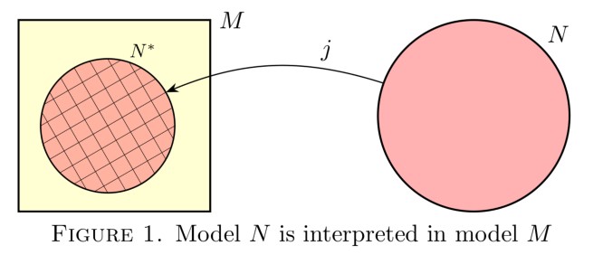

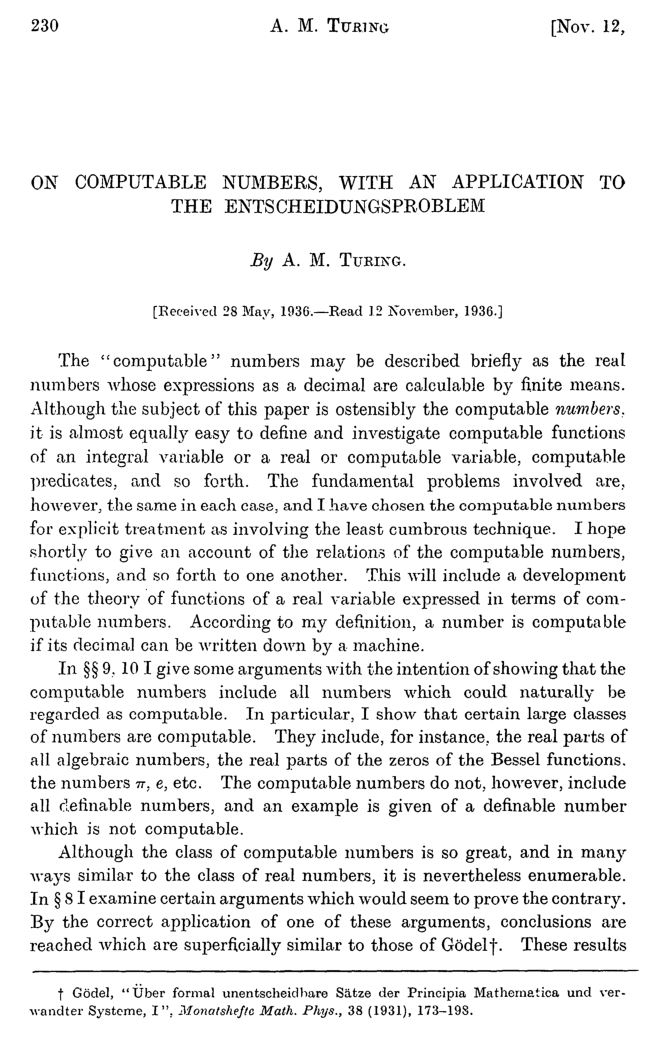
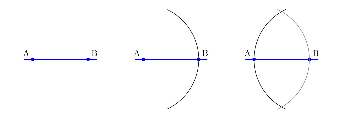


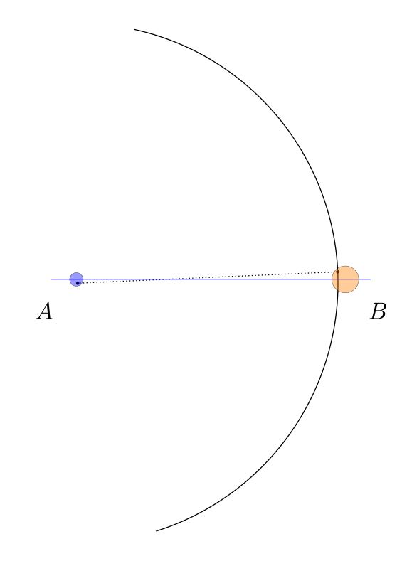
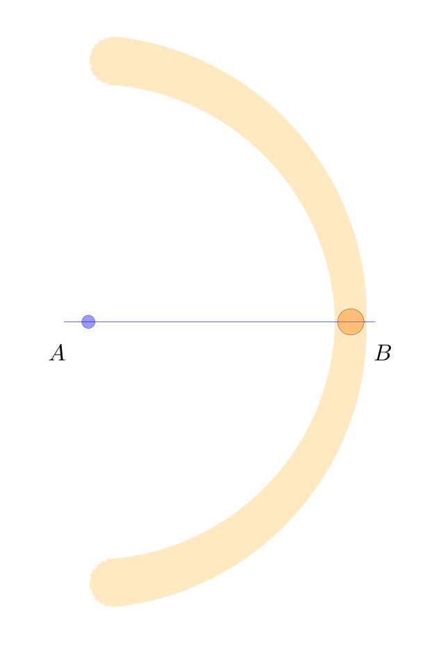


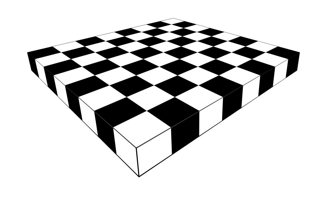

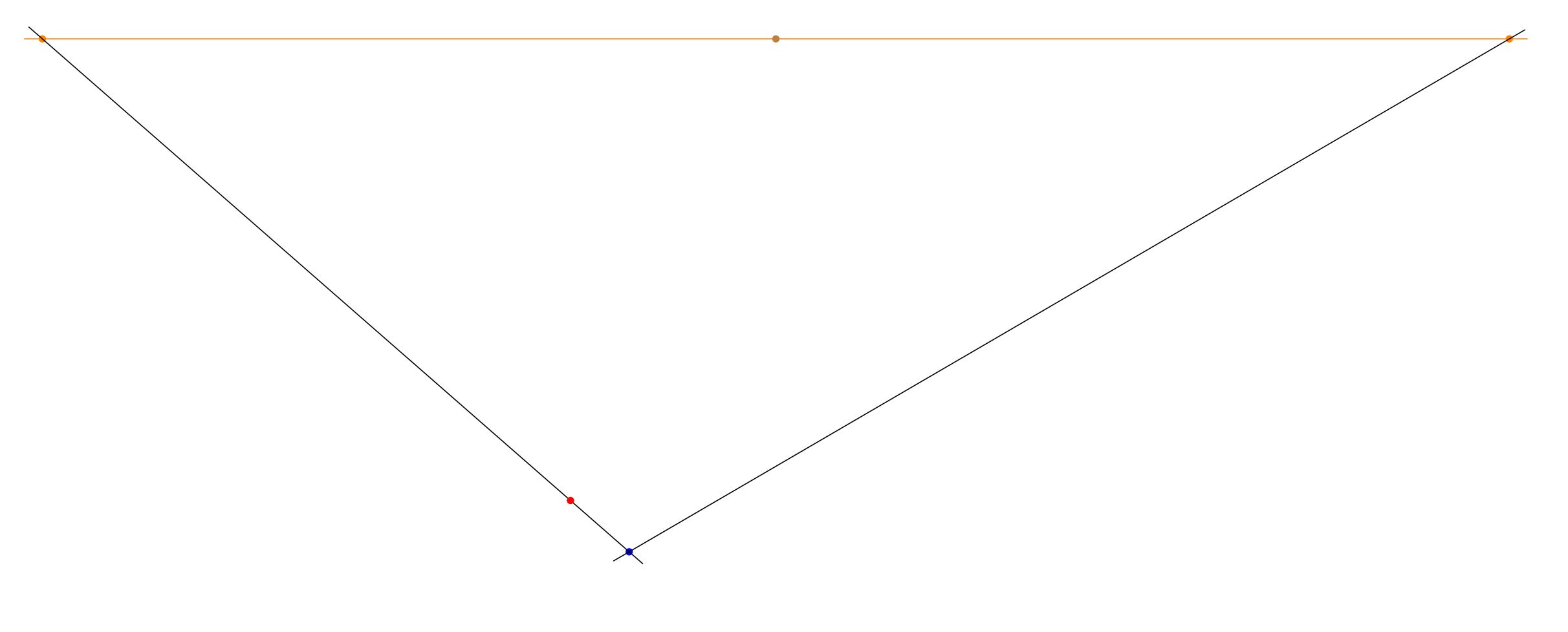


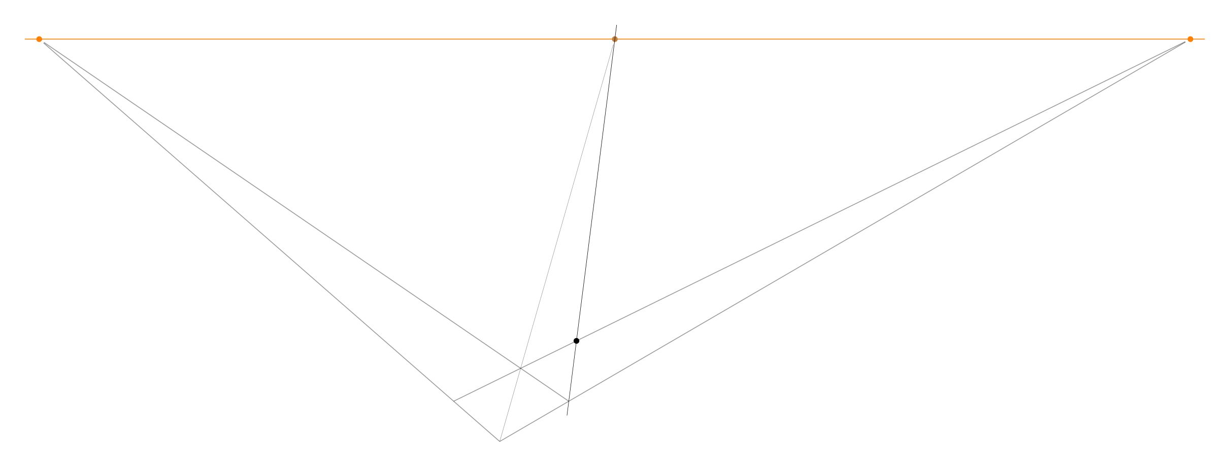


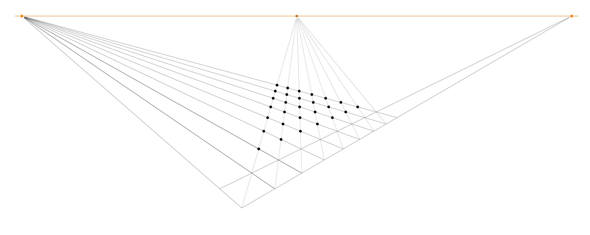

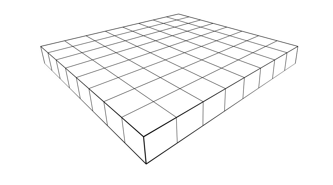
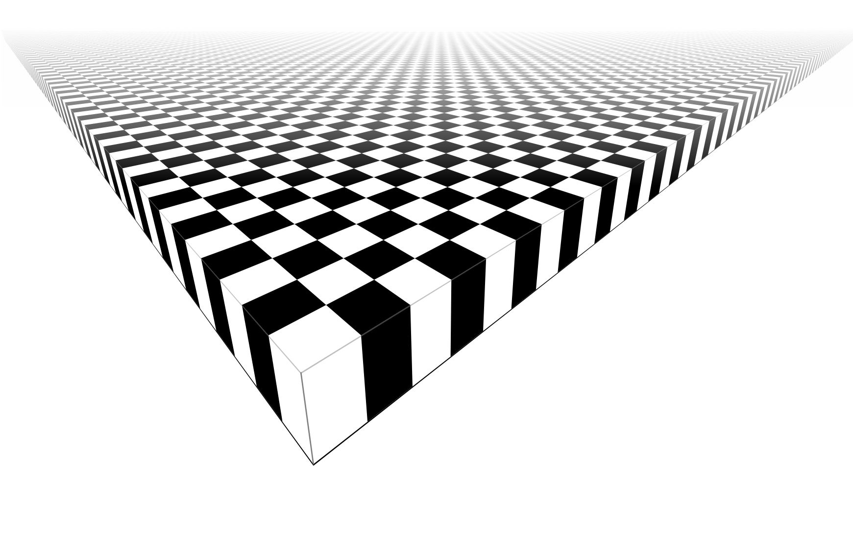
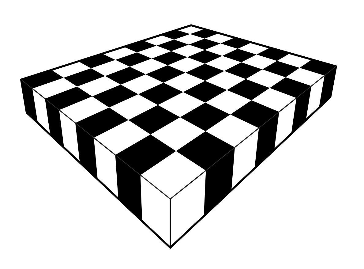
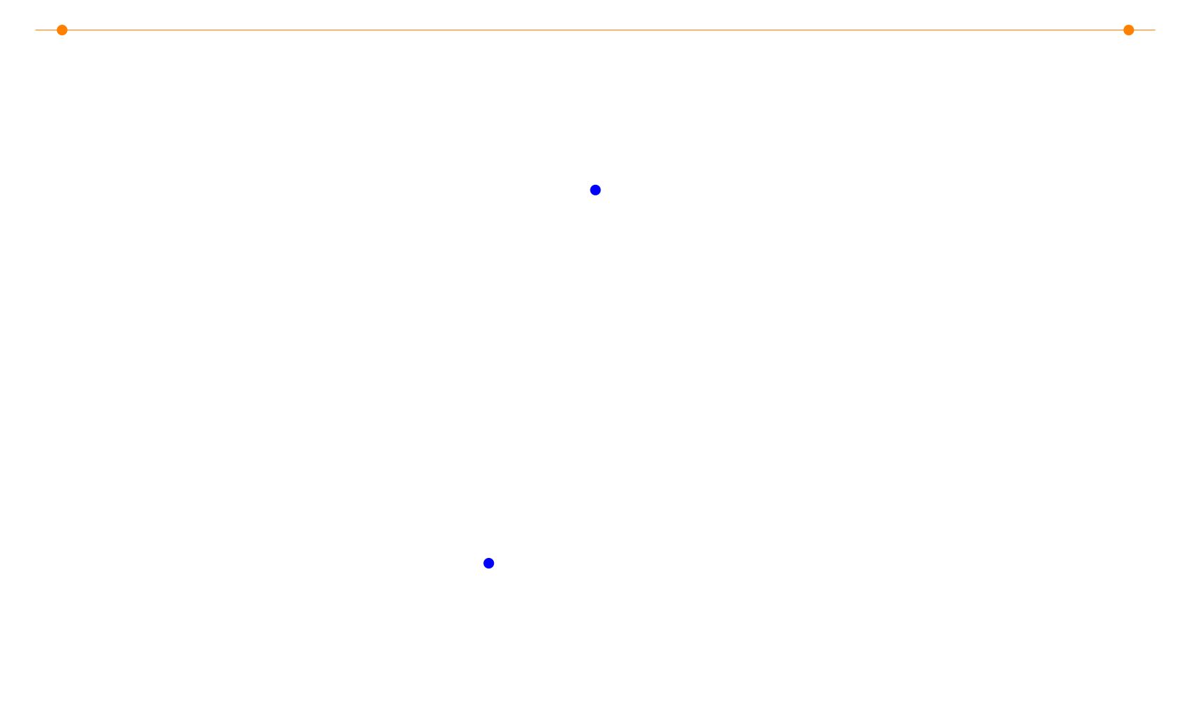

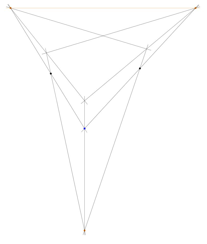


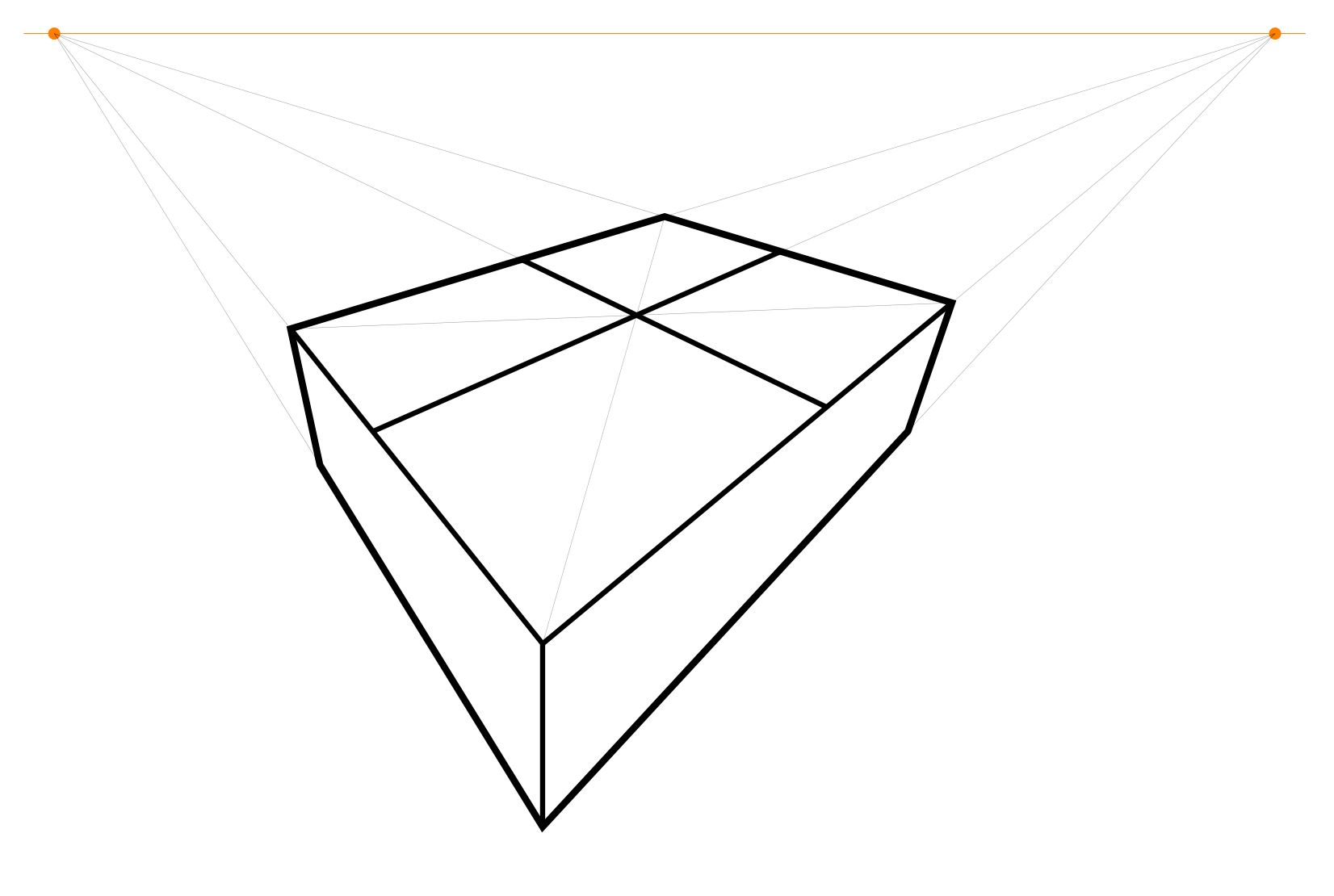

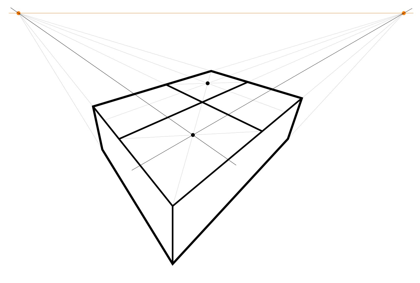
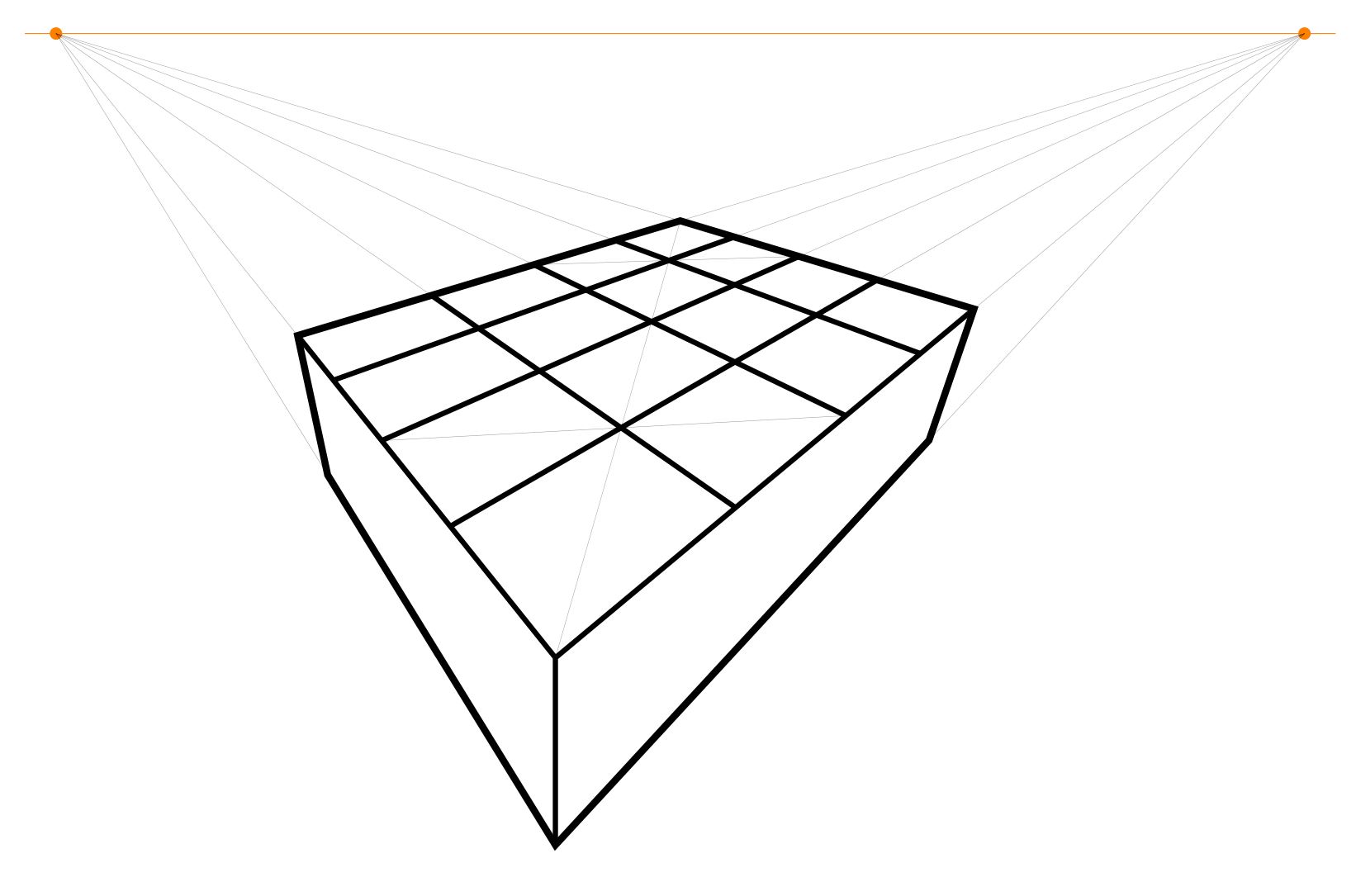

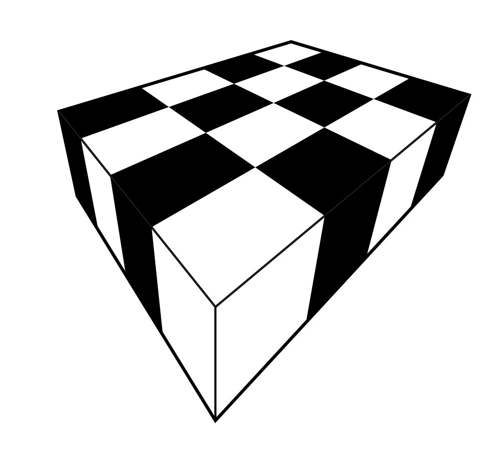

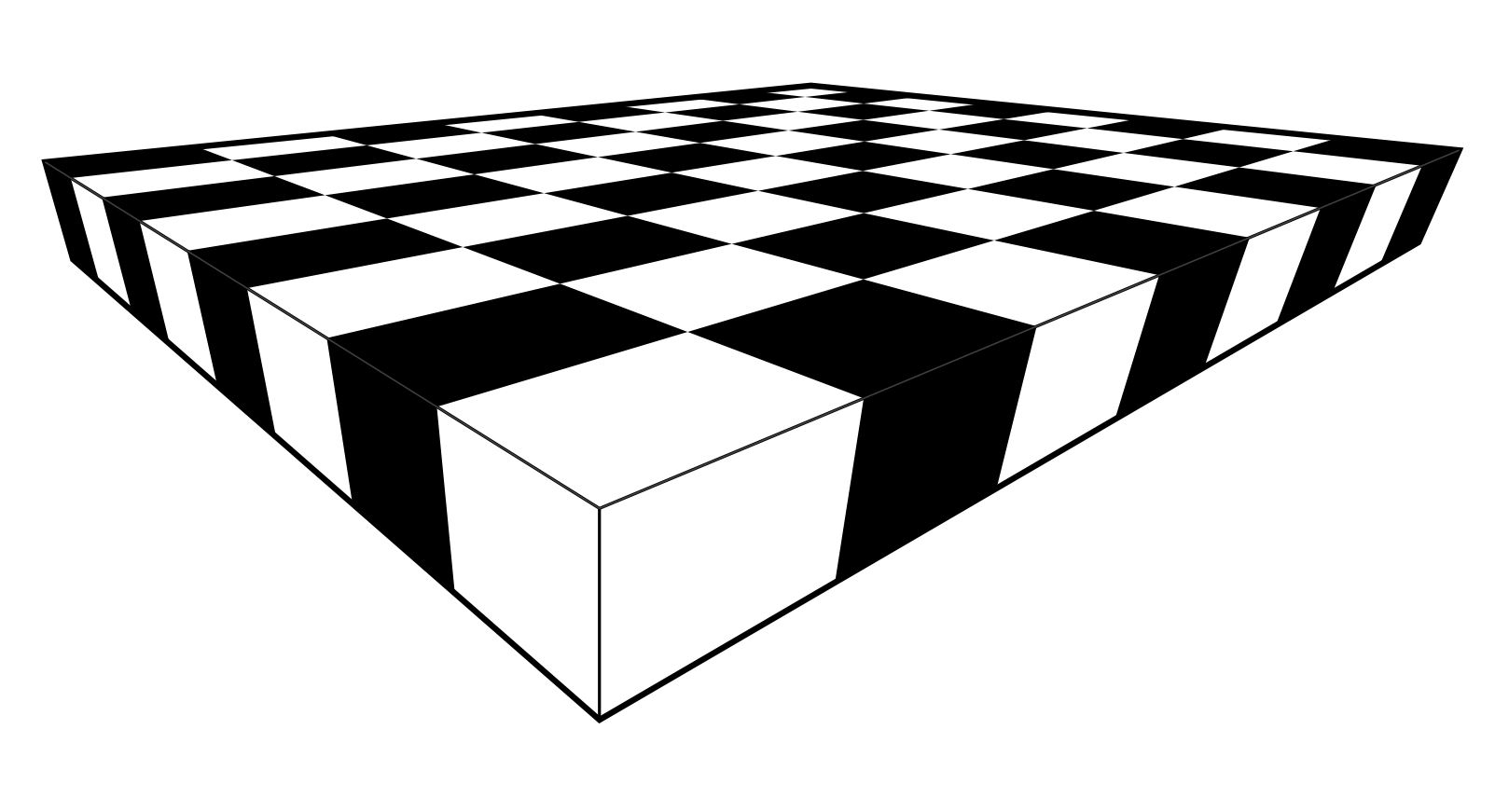
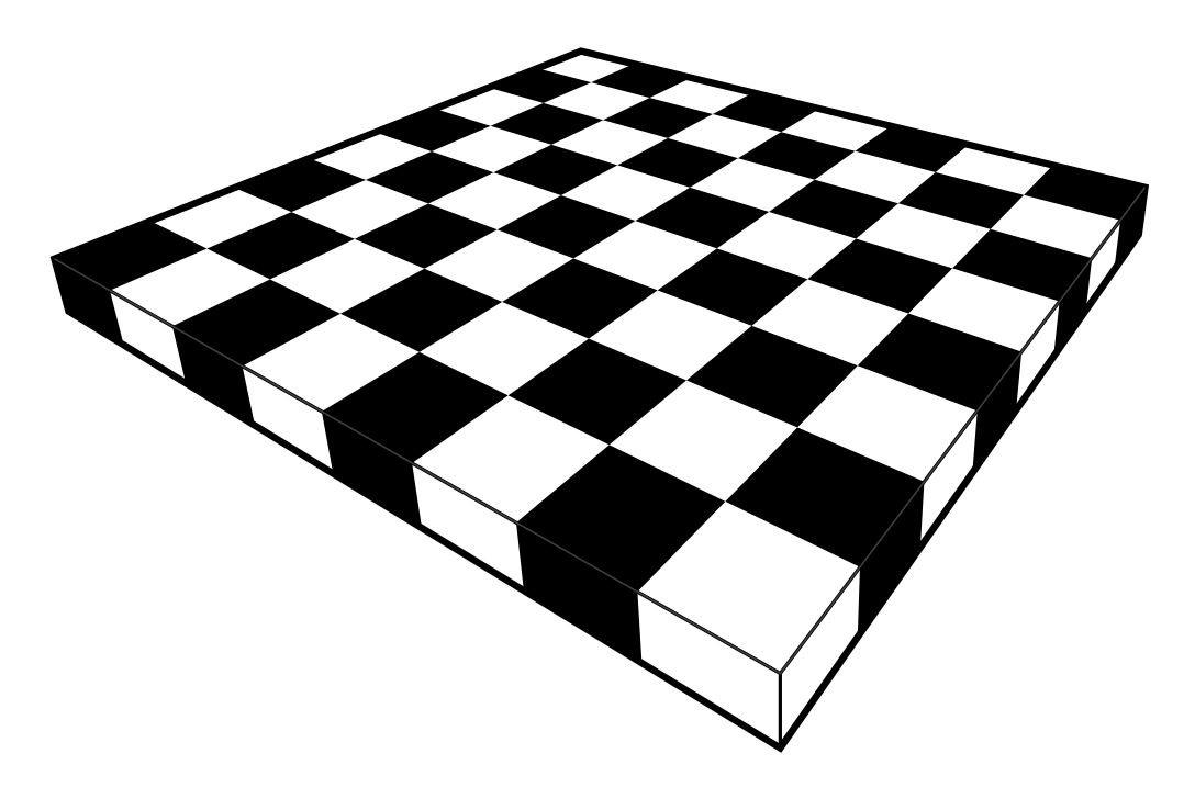
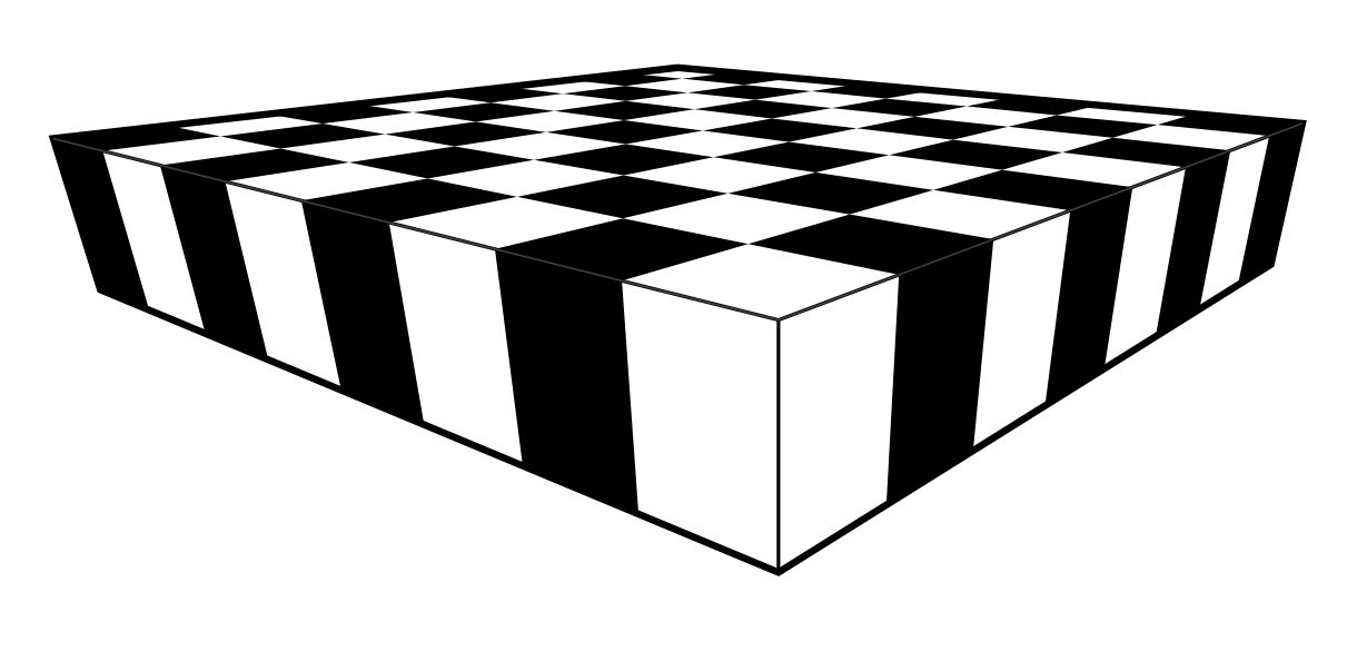
 [Public domain], via Wikimedia Commons")
 public domain image")


