A model of set theory with a definable copy of the complex field in which the two roots of -1 are set-theoretically indiscernible

Mathematicians are deeply familiar with the complex number field $\newcommand\C{\mathbb{C}}\C$, the algebraic closure of the real field $\newcommand\R{\mathbb{R}}\R$, which can be constructed from $\R$ by adjoining a new ideal element $i$, the imaginary unit, and forming the complex numbers $a+bi$ as formal pairs, defining the arithmetic subject to the rule $i^2=–1$. Thus we may add and multiply the complex numbers, according to the familiar rules:

$$(a+bi)+(c+di)=(a+c)+(b+d)i$$ $$(a+bi)\cdot(c+di)=(ac-bd)+(ad+bc)i.$$

The complex field thus provides a system of numbers giving sense to expressions like $\sqrt{–1}$, while obeying the familiar algebraic rules of a field. Hamilton had presented this conception of complex numbers as pairs of real numbers to the Royal Irish Academy in 1833.

One may easily observe in the complex numbers, however, that $–i$ is also a square root of $–1$, because

$$(–i)\cdot(–i)=(–1)^2\cdot i^2=i^2=-1.$$

Thus, both $i$ and $–i$ have the property of being square roots of $–1$, and indeed, these are the only square roots of $–1$ in the complex field.

A small conundrum may arise when one realizes that $–i$ therefore also fulfills what might have been taken as the “defining” property of the ideal element $i$, namely, that it squares to $–1$. So this property doesn’t actually define $i$, in light of the fact that there is another distinct object $–i$ that also has this property. Can we tell $i$ and $–i$ apart?

Not in the complex field, no, we cannot. The basic fact is that $i$ and $–i$ are indiscernible as complex numbers with respect to the algebraic structure of $\C$—any property that $i$ has in the structure $\langle\C,+,\cdot,0,1\rangle$ will also hold of $–i$. One way to see this is to observe that complex conjugation, the map $$a+bi\quad\mapsto\quad a-bi$$ is an automorphism of the complex number field, an isomorphism of the structure with itself. And since this automorphism swaps $i$ with $–i$, it follows that any statement true of $i$ in the complex numbers, expressible in the language of fields, will also hold of $–i$.

In fact, the complex number field $\C$ has an extremely rich automorphism group, and every irrational complex number is indiscernible from various doppelgängers. There is an automorphism of $\C$ that swaps $\sqrt{2}$ and $–\sqrt{2}$, for example, and another that permutes the cube roots of $5$, mapping the real root $\sqrt[3]{5}$ with the two nonreal roots. So these numbers can have no property not shared by their various automorphic images. The general fact is that every complex number, except the rational numbers, is moved by some automorphism of $\C$. One can begin to see this by noticing that there are two ways to embed the algebraic field extensions $\newcommand\Q{\mathbb{Q}}\Q(\sqrt{2})$ into $\C$, and both embeddings extend fully to automorphisms of $\C$.

Because there is an automorphism of $\C$ swapping $\sqrt{2}$ and $–\sqrt{2}$, it means that these two numbers are also indiscernible as complex numbers, just like $i$ and $–i$ were—any property that $\sqrt{2}$ holds in the complex numbers is also held by $–\sqrt{2}$. But wait a minute, how can that be? After all, $\sqrt{2}$ is positive and $–\sqrt{2}$ is negative, and isn’t this a property that separates them? Well, yes, in the real numbers $\R$ this is a separating property, and since the order is definable from the algebraic structure of the real field (positive numbers are exactly the nonzero squares), it is a real algebraic property that distinguishes $\sqrt{2}$ from $–\sqrt{2}$, as only the former has itself a square root in $\R$. But this definition does not work in $\C$, since both have square roots there, and more generally, the surprise is that the real numbers $\R$ are not definable as a subfield in the complex field $\C$—there is no property expressible in the language of fields that picks out exactly the real numbers. There are $2^{2^{\aleph_0}}$ many distinct ways to embed $\R$ as a subfield of $\C$, and none of them is definable in $\C$.

The conclusion is that if we regard the complex numbers with the field structure only, $\langle\C,+,\cdot,0,1\rangle$, then we cannot refer unambiguously to $i$ or $–i$, to $\sqrt{2}$ or $–\sqrt{2}$, or indeed to any irrational complex number. Every irrational number is moved by some automorphism of the complex field. The irrational algebraic numbers can be permuted in their finite sets of indiscernible roots of their irreducible polynomial, and any two transcendental complex numbers (transcendental over $\Q$) are automorphic. For example, there is an automorphism of $\C$ moving $e+2i$ to $1+\sqrt{\pi}i$.

Finding a path out of that chaos, mathematicians like to conceive of $\C$ as a field extension of $\R$, in effect fixing the copy of $\R$ in $\C$. It is as though we are working in the structure $\langle\C,+,\cdot,0,1,\R\rangle$, where we have augmented the complex field structure with a predicate picking out the real numbers. So this isn’t just a field, but a field with an identified subfield. In this structure, $\sqrt{2}$ and $\sqrt[3]{5}$ and so on are definable, since one has identified the real numbers and within that subfield the order on the reals is definable, and so we can define every real algebraic number using this order. With the predicate for $\R$ picking out the reals, the structure has only the one nontrivial automorphism, complex conjugation, and to my way of thinking, this is the reason that the indiscernibility issue is usually considered more prominently with $i$ and $–i$.

The indiscernibility of $i$ and $–i$ in the complex field has been written on at length in the philosophical literature, since it seems to refute a certain philosophical account of structuralism that might otherwise have seemed appealing. Namely, the relevant view is a version of abstract structuralism, the view that what mathematical objects are is the structural role that they play in a mathematical system. On this view the natural number $2$ simply is the role that $2$ plays in Dedekind arithmetic, the role of being the successor of the successor of zero (Dedekind arithmetic is the categorical second-order axiomatization of $\langle\newcommand\N{\mathbb{N}}\N,0,S\rangle$). The view is that what mathematical structure is is the structural roles that objects play in any instance of the structure. The structural role is exactly what is preserved by isomorphism, and so it would seem to be an invariant for the isomorphism orbits of an indidvidual with respect to a structure.

The problem with this version of abstract structuralism is that it seems to be refuted by the example of $i$ and $–i$ in the complex field. Precisely because these numbers are automorphic, they would seem each to play exactly the same role in the complex field—the two numbers are isomorphic copies of one another via complex conjugation. Thus, they are distinct numbers, but play the same structural role, and so we cannot seem to identify the abstract number with the structural roles. This problem occurs, of course, in any mathematical structure that is not rigid.

The numbers $i$ and $–i$ are indiscernible in the field structure of $\C$, but of course we can distinguish them in contexts with additional structure. For example, if we use the Hamilton presentation of the complex numbers as pairs of real numbers, representing $a+bi$ with the pair $(a,b)$, then the number $i$ has coordinates $(0,1)$ and $–i$ has coordinates $(0,-1)$. The complex field equipped with this coordinate structure, perhaps given by the real and imaginary parts operators—let us call it the complex plane, as opposed to the complex field—is a rigid structure in which $i$ and $–i$ are discernible and indeed definable.

Finally, this brings me to the main point of this blog post. What I would like to do is to prove that it is relatively consistent with ZFC that we can definably construct a copy of the complex numbers $\C$ in such a way that not only are $i$ and $–i$ indiscernible in the field structure, but actually the particular set-theoretic objects $i$ and $–i$ are indiscernible in the set-theoretic background in which the construction is undertaken.

Goal. A definable copy of the complex field in which the two square roots of $–1$ are indiscernible not only in the field structure, but also in the set-theoretic background in which the construction of the field takes place.

These two aims are in tension, for we want the particular copy $\C$ to be definable (as a particular set-theoretic object, not just defined up to isomorphism), but the individual square roots of $–1$ to be set-theoretically indiscernible.

The goal is not always possible. For example, some models of ZFC are pointwise definable, meaning that every individual set is definable in them by some distinguishing set-theoretic property. More generally, if the V=HOD axiom holds, then there is a definable global well order of the set-theoretic universe, and with any such order we could define a linear order on $\{i,–i\}$ in any definable copy of $\C$, which would allow us to define each of the roots. For these reasons, in some models of ZFC, it is not possible to achieve the goal, and the most we can hope for a consistency result.

But indeed, the consistency goal is achievable.

Theorem. If ZFC is consistent, then there is a model of ZFC that has a definable complete ordered field $\R$ with a definable algebraic closure $\C$, such that the two square roots of $–1$ in $\C$ are set-theoretically indiscernible, even with ordinal parameters.

Proof. The proof makes use of what are known as Grozek-Laver pairs, definable pair sets having no ordinal-definable element. See M. Groszek & R. Laver, Finite Groups of OD-conjugates, Periodica Mathematica Hungarica, v. 18, pp. 87–97 (1987), for a very general version of this. This theorem also appears at theorem 4.6 in my paper Ehrenfeucht’s lemma in set theory, joint with Gunter Fuchs, Victoria Gitman, and myself. The arguments provide a model of set theory with a definable pair set $A=\{i,j\}$, such that neither element $i$ nor $j$ is definable from ordinal parameters. The pair set is definable, but neither element is definable.

To undertake the construction, we start with one of the standard definable constructions of the real field $\R$. For example, we could use Dedekind cuts in $\Q$, where $\Q$ is constructed explicitly as the quotient field of the integer ring $\mathbb{Z}$ in some canonical definable manner, and where the integers are definably constructed from a definable copy of the natural numbers $\mathbb{N}$, such as the finite von Neumann ordinals. So we have a definable complete ordered field, the real field $\R$.

Given this and the set $A$, we follow a suggestion of Timothy Gowers in the discussion of this problem on Twitter. Namely, we use the elements of $A$ as variables to form the polynomial ring $\R[A]$, meaning $\R[i,j]$, where $i$ and $j$ are the two elements of $A$. It is not necessary to distinguish the elements of $A$ to form this ring of polynomials, since we take all finite polynomial expressions using real coefficients and elements of $A$ raised to a power. (In particular, although I have referred to the elements as $i$ and $j$, there is to be no suggestion that I am somehow saying $i$ is the “real” $i$; I am not, for I could have called them $j$,$i$ or $j$,$k$ or $a$,$a’$, and so on.) Then we quotient by the ideal $(i^2+1,i+j)$, which is defined symmetrically in the elements of $A$, since it is the same ideal as $(j^2+1,j+i)$. Let $\C$ be the quotient $\C=\R[i,j]/(i^2+1,i+j)$, which will make both $i$ and $j$ the two square roots of $–1$, and so by the fundamental theorem of algebra this is a copy of the complex numbers.

Since $\R$ and $A$ were definable, and we didn’t need ever to choose a particular element of $A$ in the construction to define the polynomial ring or the ideal, this copy of $\C$ is definable without parameters. But since $i$ and $j$ are set-theoretically indiscernible in the model of set theory in which we are undertaking the construction, it follows that their equivalence classes in the quotient are also indiscernible. And so we have a definable copy of the complex field $\C$, extending a definable copy of $\R$, in which the two square roots of $–1$ are indiscernible not just in the field structure, but fully in the set-theoretic background in which the fields were constructed. $\Box$

In particular, in this model of set theory, there will be absolutely no way to distinguish the two roots by any further definable structure, whether using second-order or higher-order definitions of the field $\C$ or using any definable set-theoretic property whatsoever.

The analysis suggests a natural further inquiry. Namely,

Question. Is there a model of set theory with a definable copy of the complex field $\C$, such that the hierarchy of relative definability and indiscernibility in $\C$ matches the set-theoretic relative definability and indiscernibility of the objects?

That is, we would want to mimic the phenomenon of $i$ and $–i$ in the above construction with all complex numbers, so that $\sqrt{2}$ and $–\sqrt{2}$ were also indiscernible, not just in this copy of $\C$ but also in the set-theoretic background, and $\sqrt[4]{2}$ was set-theoretically indiscernible from the other new fourth-root of $2$, but can set-theoretically define both $\sqrt{2}$ and $–\sqrt{2}$. In other words, I want the set-theoretic definability hierarchy to match the complex-number-theoretic definability hierarchy. I may post this question on MathOverflow, when I formulate a version of it with which I am satisfied. I believe it will be answered by iterated Sacks forcing in a manner similar to that used in many papers by Marcia Groszek, and in particular, in my paper with her, The Implicitly constructible universe.

The sentence asserting its own non-forceability by nontrivial forcing

At the meeting here in Konstanz, Giorgo Venturi and I considered the sentence $\sigma$, which asserts its own non-forceability by nontrivial forcing. That is, $\sigma$ asserts that there is no nontrivial forcing notion forcing $\sigma$. $$\sigma\quad\iff\quad \neg\exists\mathbb{B}\ \Vdash_{\mathbb{B}}\sigma.$$ The sentence $\sigma$ would be a fixed-point of the predicate for not being nontrivially forceable.

In any model of set theory $V$ in which $\sigma$ is true, then in light of what it asserts, it would not be forceable by nontrivial forcing, and so it would be false in all nontrivial forcing extensions of that model $V[G]$. And in any model $W$ where it is false, then because of what it asserts, it would be nontrivially forceable, and so it would be true in some forcing extension of that model $W[G]$.

But this is a contradiction! It cannot ever be true, since if it were true in $V$, it would have to be false in all extensions $V[G]$, and therefore true in some subsequent extension $V[G][H]$. But that model is a forcing extension of $V$, contradicting the claim that it is false in all such extensions.

So it must always be false, but this can’t happen, since then in any given model, in light of what it asserts, it would have to be true. So it cannot ever be true or false.

Conclusion: there is no such sentence σ that asserts its own nontrivial forceability. This is no fixed-point for not being nontrivially forceable.

But doesn’t this contradict the fixed-point lemma? After all, the fixed-point lemma shows that we can produce fixed points for any expressible assertion.

The resolution of the conundrum is that although for any given assertion $\varphi$, we can express “$\varphi$ is forceable”, we cannot express “x is the Gödel code of a forceable sentence”, for reasons similar to those for Tarski’s theorem on the nondefinability of truth.

Therefore, we are not actually in a situation to apply the fixed-point lemma. And ultimately the argument shows that there can be no sentence $\sigma$ that asserts “$\sigma$ is not forceable by nontrivial forcing”.

Ultimately, I find the logic of this sentence $\sigma$, asserting its own non-nontrivial forceability, to be a set-theoretic forcing analogue of the Yablo paradox. The sentence holds in a model of set theory whenever it fails in all subsequent models obtained by forcing, and that relation is exactly what arises in the Yablo paradox.

Quantifer elimination

A theory admits quantifier-elimination when every assertion is logically equivalent over the theory to a quantifier-free assertion. This is quite a remarkable property when it occurs, because it reveals a severe limitation on the range of concepts that can be expressed in the theory—a quantifier-free assertion, after all, is able to express only combinations of the immediate atomic facts at hand. As a result, we are generally able to prove quantifier-elimination results for a theory only when we already have a profound understanding of it and its models, and the quantifier-elimination result itself usually leads quickly to classification of the definable objects, sets, and relations in the theory and its models. In this way, quantifier-elimination results often showcase our mastery over a particular theory and its models. So let us present a few quantifier-elimination results, exhibiting our expertise over some natural theories.

Endless dense linear orders

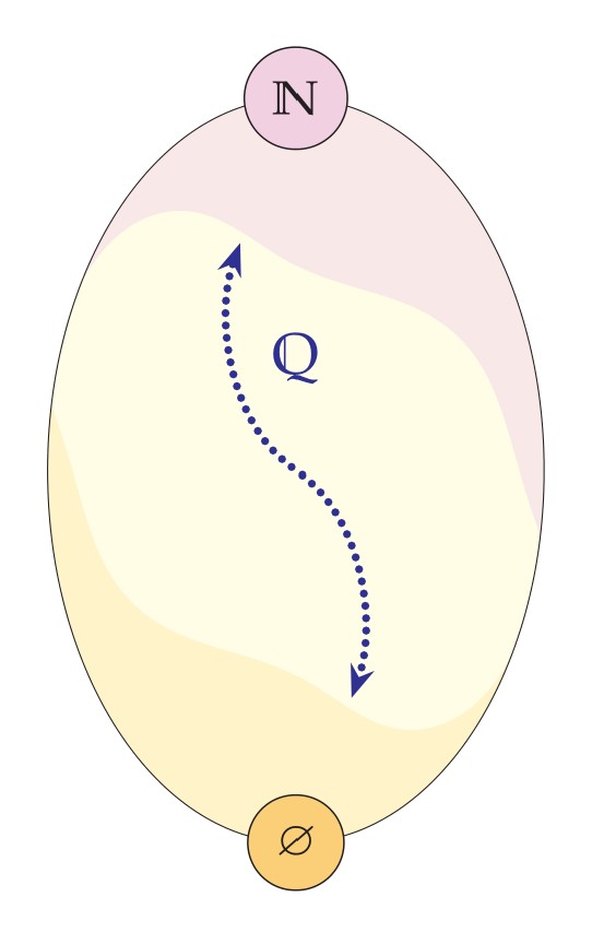
$\def\<#1>{\left\langle#1\right\rangle}\newcommand\Q{\mathbb{Q}}\newcommand\R{\mathbb{R}}\newcommand\N{\mathbb{N}}\newcommand\bottom{\mathord{\perp}}\newcommand{\Th}{\mathop{\rm Th}}\newcommand{\unaryminus}{-}\newcommand\Z{\mathbb{Z}}\newcommand\divides{\mid}$Consider first the theory of an endless dense linear order, such as the rational order $\<\Q,<>$. In light of Cantor’s theorems on the universality of the rational line and the categoricity theorem for countable endless dense linear orders, we already have a fairly deep understanding of this theory and this particular model.

Consider any two rational numbers $x,y$ in the structure $\<\Q,<>$. What can one say about them? Well, we can certainly make the atomic assertions that $x$ to a Boolean combination of these assertions.

Theorem. The theory of the rational order $\<\Q,<>$ admits elimination of quantifiers—every assertion $\varphi(x,\ldots)$ is logically equivalent in the rational order to a quantifier-free assertion.

Proof. To see this, observe simply by Cantor’s categoricity theorem for countable dense linear orders that any pair $x<y$ in $\Q$ is automorphic to any other such pair $x'<y’$, and similarly for pairs with $x=y$ or $y<x$. Consequently, $\varphi(x,y)$ either holds of all pairs with $x<y$ or of none of them, of all pairs with $x=y$ or none, and of all pairs with $y<x$ or none. The assertion $\varphi(x,y)$ is therefore equivalent to the disjunction of the three atomic relations for which it is realized, including $\top$ as the disjunction of all three atomic possibilities and $\bottom$ as the empty disjunction.

More generally, a similar observation applies to assertions $\varphi(x_1,\ldots,x_n)$ with more free variables. By Cantor’s theorem, every $n$-tuple of points in $\Q$ is automorphic with any other such $n$-tuple of points having the same atomic order relations. Therefore any assertion holding of one such $n$-tuple holds of all $n$-tuples with that same atomic type, and consequently every assertion $\varphi(x_1,\ldots,x_n)$ is logically equivalent in $\<\Q,<>$ to a disjunction of those combinations of atomic relations amongst the variables $x_1,\ldots,x_n$ for which it holds. In particular, every assertion is equivalent in $\<\Q,<>$ to a quantifier-free assertion. In short, the theory of this model $\Th(\<\Q,<>)$ admits elimination of quantifiers. $\Box$

What about other endless dense linear orders? The argument we have given so far is about the theory of this particular model $\<\Q,<>$. In fact, the theory of the rational order is exactly the theory of endless dense linear orders, because this theory is complete, which one can see as an immediate consequence of the categoricity result of Cantor’s theorem and the downward Löwenheim-Skolem theorem. In my book, I have not yet proved the Löwenheim-Skolem theorem at this stage, however, and so let me give a direct proof of quantifier-elimination in the theory of endless dense linear orders, from which we can also derive the completeness of this theory.

Theorem. In the theory of endless dense linear orders, every statement is logically equivalent to a quantifier-free statement.

Proof. To clarify, the quantifier-free statement will have the same free variables as the original assertion, provided we allow $\bottom$ and $\top$ as logical constants. We argue by induction on formulas. The claim is of course already true for the atomic formulas, and it is clearly preserved under Boolean connectives. So it suffices inductively to eliminate the quantifier from $\exists x\, \varphi(x,\ldots)$, where $\varphi$ is itself quantifier-free. We can place $\varphi$ in disjunctive normal form, a disjunction of conjunction clauses, where each conjunction clause is a conjunction of literals, that is, atomic or negated atomic assertions. Since the atomic assertions $x<y$, $x=y$ and $y<x$ are mutually exclusive and exhaustive, the negation of any one of them is equivalent to the disjunction of the other two. Thus we may eliminate any need for negation. By redistributing conjunction over disjunction as much as possible, we reduce to the case of $\exists x\,\varphi$, where $\varphi$ is in disjunctive normal form without any negation. The existential quantifier distributes over disjunction, and so we reduce to the case $\varphi$ is a conjunction of atomic assertions. We may eliminate any instance of $x=x$ or $y=y$, since these impose no requirement. We may assume that the variable $x$ occurs in each conjunct, since otherwise that conjunct commutes outside the quantifier. If $x=y$ occurs in $\varphi$ for some variable $y$ not identical to $x$, then the existential claim is equivalent to $\varphi(y,\ldots)$, that is, by replacing every instance of $x$ with $y$, and we have thus eliminated the quantifier. If $x<x$ occurs as one of the conjuncts, this is not satisfiable and so the assertion is equivalent to $\bottom$. Thus we have reduced to the case where $\varphi$ is a conjunction of assertions of the form $x<y_i$ and $z_j<x$. If only one type of these occurs, then the assertion $\exists x\,\varphi$ is outright provable in the theory by the endless assumption and thus equivalent to $\top$. Otherwise, both types $x<y_i$ and $z_j<x$ occur, and in this case the existence of an $x$ obeying this conjunction of assertions is equivalent over the theory of endless dense linear orders to the quantifier-free conjunction $\bigwedge_{i,j}z_j<y_i$, since there will be an $x$ between them in this case and only in this case. Thus, we have eliminated the quantifier $\exists x$, and so by induction every formula is equivalent over this theory to a quantifier-free formula. $\Box$

Corollary. The theory of endless dense linear orders is complete.

Proof. If $\sigma$ is any sentence in this theory, then by theorem above, it is logically equivalent to a Boolean combination of quantifier-free assertions with the same variables. Since $\sigma$ is a sentence and there are no quantifier-free atomic sentences except $\bottom$ and $\top$, it follows that $\sigma$ is equivalent over the theory to a Boolean combination of $\bottom$ or $\top$. All such sentences are equivalent either to $\bottom$ or $\top$, and thus either $\sigma$ is entailed by the theory or $\neg\sigma$ is, and so the theory is complete. $\Box$

Corollary. In any endless dense linear order, the definable sets (allowing parameters) are precisely the finite unions of intervals.

Proof. By intervals we mean a generalized concept allowing either open or closed endpoints, as well as rays, in any of the forms:
$$(a,b)\qquad [a,b]\qquad [a,b)\qquad (a,b]\qquad (a,\infty)\qquad [a,\infty)\qquad (\unaryminus\infty,b)\qquad (\unaryminus\infty,b]$$
Of course any such interval is definable, since $(a,b)$ is defined by $(a<x)\wedge(x<b)$, taking the endpoints $a$ and $b$ as parameters, and $(-\infty,b]$ is defined by $(x<b)\vee (x=b)$, and so on. Thus, finite unions of intervals are also definable by taking a disjunction.

Conversely, any putative definition $\varphi(x,y_1,\ldots,y_n)$ is equivalent to a Boolean combination of atomic assertions concerning $x$ and the parameters $y_i$. Thus, whenever it is true for some $x$ between, above, or below the parameters $y_i$, it will be true of all $x$ in that same interval, and so the set that is defined will be a finite union of intervals having the parameters $y_i$ as endpoints, with the intervals being open or closed depending on whether the parameters themselves satisfy the formula or not. $\Box$

Theory of successor

Let us next consider the theory of a successor function, as realized for example in the Dedekind model, $\<\N,S,0>$, where $S$ is the successor
function $Sn=n+1$. The theory has the following three axioms:
$$\forall x\, (Sx\neq 0)$$

$$\forall x,y\, (Sx=Sy\implies x=y)$$

$$\forall x\, \bigl(x\neq 0\implies \exists y\,(Sy=x)\bigr).$$
In the Dedekind model, every individual is definable, since $x=n$ just in case $x=SS\cdots S0$, where we have $n$ iterative applications of $S$. So this is a pointwise definable model, and hence also Leibnizian. Note the interplay between the $n$ of the object theory and $n$ of the metatheory in the claim that every individual is definable.

What definable subsets of the Dedekind model can we think of? Of course, we can define any particular finite set, since the numbers are definable as individuals. For example, we can define the set ${1,5,8}$ by saying, “either $x$ has the defining property of $1$ or it has the defining property of $5$ or it has the defining property of $8$.” Thus any finite set is definable, and by negating such a formula, we see also that any cofinite set—the complement of a finite set—is definable. Are there any other definable sets? For example, can we define the set of even numbers? How could we prove that we cannot? The Dedekind structure has no automorphisms, since all the individuals are definable, and so we cannot expect to use automorphism to show that the even numbers are not definable as a set. We need a deeper understanding of definability and truth in this structure.

Theorem. The theory of a successor function admits elimination of quantifiers—every assertion is equivalent in this theory to a quantifier-free assertion.

Proof. By induction on formulas. The claim is already true for atomic assertions, since they have no quantifiers, and quantifier-free assertions are clearly closed under the Boolean connectives. So it suffices by induction to eliminate the quantifier from assertions of the form $\exists x\, \varphi(x,\ldots)$, where $\varphi$ is quantifier free. We may place $\varphi$ in disjunctive normal form, and since the quantifier distributes over disjunction, we reduce to the case that $\varphi$ is a conjunction of atomic and negated atomic assertions. We may assume that $x$ appears in each atomic conjunct, since otherwise we may bring that conjunct outside the quantifier. We may furthermore assume that $x$ appears on only one side of each atomic clause, since otherwise the statement is either trivially true as with $SSx=SSx$ or $Sx\neq SSx$, or trivially false as with $Sx=SSx$. Consider for example:
$$\exists x\,\bigl[(SSSx=y)\wedge (SSy=SSSz)\wedge (SSSSSx=SSSw)\wedge{}$$
$$\hskip1in{}\wedge (Sx\neq SSSSw)\wedge (SSSSy\neq SSSSSz)\bigr]$$
We can remove duplicated $S$s occurring on both sides of an equation. If $x=S^ky$ appears, we can get rid of $x$ and replace all occurrences with $S^ky$. If $S^nx=y$ appears, can add $S$’s everywhere and then replace any occurrence of $S^nx$ with $y$. If only inequalities appear, then the statement is simply true.

For example, since the third clause in the formula above is equivalent to $SSx=w$, we may use that to omit any need to refer to $x$, and the formula overall is equivalent to
$$(Sw=y)\wedge (y=Sz)\wedge (w\neq SSSSSw)\wedge (y\neq Sz),$$ which has no quantifiers.
Since the method is completely general, we have proved that the theory of successor admits elimination of quantifiers. $\Box$

It follows that the definable sets in the Dedekind model $\<\N,S,0>$, using only the first-order language of this structure, are precisely the finite and cofinite sets.

Corollary. The definable sets in $\<\N,S,0>$ are precisely the finite and cofinite sets

Proof. This is because an atomic formula defines a finite set, and the collection of finite or cofinite sets is closed under negation and Boolean combinations. Since every formula is equivalent to a quantifier-free formula, it follows that every formula is a Boolean combination of atomic formulas, and hence defines a finite or cofinite set. $\Box$

In particular, the concepts of being even or being odd are not definable from the successor operation in $\<\N,S,0>$, since the set of even numbers is neither finite nor cofinite.

Corollary. The theory of a successor function is complete—it is the theory of the standard model $\<\N,S,0>$.

Proof. If $\sigma$ is a sentence in the language of successor, then by the quantifier-elimination theorem it is equivalent to a quantifier-free assertion in the language with the successor function $S$ and constant symbol $0$. But the only quantifier-free sentences in this language are Boolean combinations of equations of the form $S^n0=S^k0$. Since all such equations are settled by the theory, the sentence itself is settled by the theory, and so the theory is complete. $\Box$

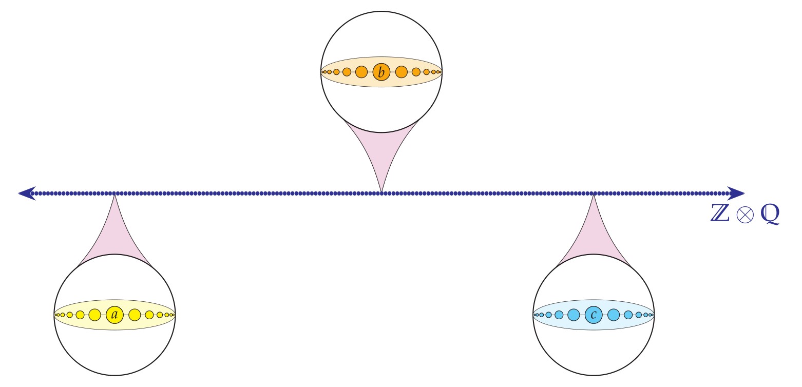
We saw that the three axioms displayed on the previous page were true in the Dedekind model $\<\N,S,0>$. Are there any other models of these axioms? Yes, there are. For example, we can add another $\Z$-chain of successors on the side, as with $\N+\Z$ or $\N\sqcup\Z$, although we shall see that the order is not definable. What are the definable elements in the enlarged structure? Still $0$ and all its finite successors are definable as before. But no elements of the $\Z$-chains can be definable, because we may perform an automorphism of the structure that translates elements within the $\Z$-chain by a fixed amount.

Let me prove next that the theory implies the induction axiom schema.

Corollary. The theory of successor (the three axioms) implies the induction axiom schema in the language of successor, that is, the following assertion for any assertion $\varphi(x)$:
$$\left[\varphi(0)\wedge\bigl(\forall x\,\bigl(\varphi(x)\implies\varphi(Sx)\bigr)\right]\implies\forall x\,\varphi(x)$$

Proof. Consider the set defined by $\varphi(x)$. By the earlier corollary, it must be eventually periodic in the standard model $\<\N,S,0>$. But by the induction assumption stated in the theorem, it must hold of every number in the standard model. So the standard model thinks that $\forall x\,\varphi(x)$. But the theory of the standard model is the theory of successor, which is complete. So the theory of successor entails that $\varphi$ is universal, as desired. $\Box$

In other words, in the trivial theory of successor–the three axioms—we get the corresponding induction axiom for free.

Presburger arithmetic

Presburger arithmetic is the theory of addition on the natural numbers, that is, the theory of the structure $\<\N,+,0,1>$. The numbers $0$ and $1$ are actually definable here from addition alone, since $0$ is the unique additive identity, and $1$ is the only number $u$ that is not expressible as a sum $x+y$ with both $x\neq u$ and $y\neq u$. So we may view this model if desired as a definitional expansion of $\<\N,+>$, with addition only. The number $2$ is similarly definable as $1+1$, and indeed any number $n$ is definable as $1+\cdots+1$, with $n$ summands, and so this is a pointwise definable model and hence also Leibnizian.

What are the definable subsets? We can define the even numbers, of course, since $x$ is even if and only if $\exists y\,(y+y=x)$. We can similarly define congruence modulo $2$ by $x\equiv_2 y\iff \exists z\,\bigl[(z+z+x=y)\vee (z+z+y=x)\bigr]$. More generally, we can express the relation of congruence modulo $n$ for any fixed $n$ as follows:
$$x\equiv_n y\quad\text{ if and only if }\exists z\,\bigl[(\overbrace{z+\cdots+z}^n+x=y)\vee(\overbrace{z+\cdots+z}^n+y=x)\bigr].$$
What I claim is that this exhausts what is expressible.

Theorem. Presburger arithmetic in the definitional expansion with all congruence relations, that is, the theory of the structure
$$\<\N,+,0,1,\equiv_2,\equiv_3,\equiv_4,\ldots>$$
admits elimination of quantifiers. In particular, every assertion in the language of $\<\N,+,0,1>$ is equivalent to a quantifer-free assertion in the language with the congruence relations.

Proof. We consider Presburger arithmetic in the language with addition $+$, with all the congruence relations $\equiv_n$ for every $n\geq 2$, and the constants $0$ and $1$. We prove quantifier-elimination in this language by induction on formulas. As before the claim already holds for atomic assertions and is preserved by Boolean connectives. So it suffices to eliminate the quantifier from assertions of the form $\exists x\,\varphi(x,\ldots)$, where $\varphi$ is quantifier-free. By placing $\varphi$ into disjunctive normal form and distributing the quantifier over the disjunction, we may assume that $\varphi$ is a conjunction of atomic and negated atomic assertions. Note that negated congruences are equivalent to a disjunction of positive congruences, such as in the case:
$$x\not\equiv_4 y\quad\text{ if and only if }\quad (x+1\equiv_4y)\vee(x+1+1\equiv_4y)\vee (x+1+1+1\equiv_4 y).$$
We may therefore assume there are no negated congruences in $\varphi$. By canceling like terms on each side of an equation or congruence, we may assume that $x$ occurs on only one side. We may assume that $x$ occurs nontrivially in every conjunct of $\varphi$, since otherwise this conjunct commutes outside the quantifier. Since subtraction modulo $n$ is the same as adding $n-1$ times, we may also assume that all congruences occurring in $\varphi$ have the form $kx\equiv_n t$, where $kx$ denotes the syntactic expression $x+\cdots+x$ occurring in the formula, with $k$ summands, and $t$ is a term not involving the variable $x$. Thus, $\varphi$ is a conjunction of expressions each having the form $kx\equiv_n t$, $ax+r=s$, or $bx+u\neq v$, where $ax$ and $bx$ similarly denote the iterated sums $x+\cdots+x$ and $r,s,u,v$ are terms not involving $x$.

If indeed there is a conjunct of the equality form $ax+r=s$ occurring in $\varphi$, then we may omit the quantifier as follows. Namely, in order to fulfill the existence assertion, we know that $x$ will have to solve $ax+r=s$, and so in particular $r\equiv_a s$, which ensures the existence of such an $x$, but also in this case any inequality $bx+u\neq v$ can be equivalently expressed as $abx+au\neq av$, which since $ax+r=s$ is equivalent to $bs+au\neq av+br$, and this does does not involve $x$; similarly, any congruence $kx\equiv_n t$ is equivalent to $akx\equiv_{an}at$, which is equivalent to $s\equiv_{an} r+at$, which again does not involve $x$. Thus, when there is an equality involving $x$ present in $\varphi$, then we can use that fact to express the whole formula in an equivalent manner not involving $x$.

So we have reduced to the case $\exists x\,\varphi$, where $\varphi$ is a conjunction of inequalities $bs+u\neq v$ and congruences $kx\equiv_n t$. We can now ignore the inequalities, since if the congruence system has a solution, then it will have infinitely many solutions, and so there will be an $x$ solving any finitely given inequalities. So we may assume that $\varphi$ is simply a list of congruences of the form $kx\equiv_n t$, and the assertion is that this system of congruences has a solution. But there are only finitely many congruences mentioned, and so by working modulo the least common multiple of the bases that occur, there are only finitely many possible values for $x$ to be checked. And so we can simply replace $\varphi$ with a disjunction over these finitely many values $i$, replacing $x$ in each conjunction with $1+\cdots+1$, using $i$ copies of $1$, for each $i$ up to the least common multiples of the bases that arise in the congruences appearing in $\varphi$. If there is an $x$ solving the system, then one of these values of $i$ will work, and conversely.

So we have ultimately succeeded in expressing $\exists x\,\varphi$ in a quantifier-free manner, and so by induction every assertion in Presburger arithmetic is equivalent to a quantifier-free assertion in the language allowing addition, congruences, and the constants $0$ and $1$. $\Box$

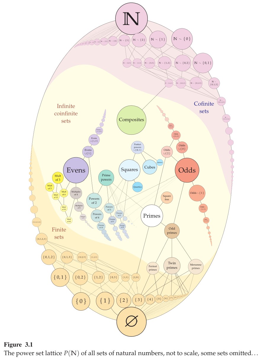
Corollary. The definable sets in $\<\N,+,0,1>$ are exactly the eventually periodic sets.

Proof. Every periodic set is definable, since one can specify the set up to the period $p$, and then express the invariance modulo $p$. Any finite deviation from a definable set also is definable, since every individual number is definable. So every eventually period set is definable. Conversely, every definable set is defined by a quantifier-free assertion in the language of $\<\N,+,0,1,\equiv_2,\equiv_3,\equiv_4,\ldots>$. We may place the definition in disjunctive normal form, and again replace negated congruences with a disjunction of positive congruences. For large enough values of $x$, the equalities and inequalities appearing in the definition become irrelevant, and so the definition eventually agrees with a finite union of solutions of congruence systems. Every such system is periodic with a period at most the least common multiple of the bases of the congruences appearing in it. And so every definable set is eventually periodic, as desired. $\Box$

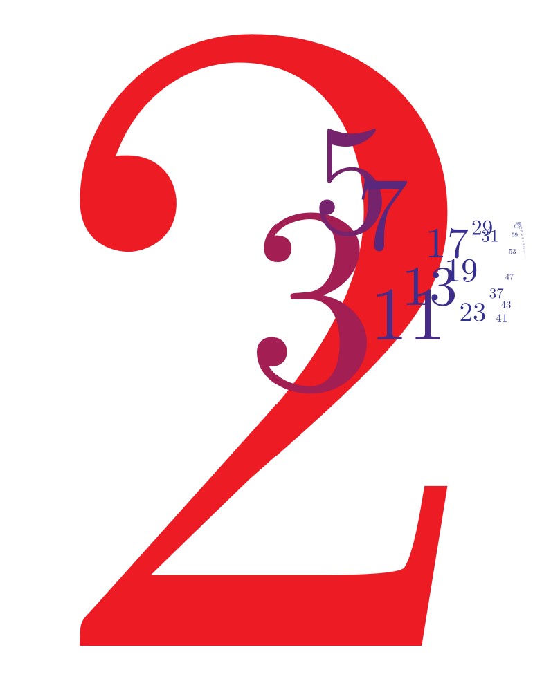
Corollary. Multiplication is not definable in $\<\N,+,0,1>$. Indeed, the squaring operation is not definable, and neither is the divisibility relation $p\divides q$.

Proof. If we could define multiplication, or even the squaring operation, then we would be able to define the set of perfect squares, but this is not eventually periodic. Similarly, if we could define the divides relation $p\divides q$, then we could define the set of prime numbers, which is not eventually periodic. $\Box$

Real-closed field

Let us lastly consider the ordered real field $\<\R,+,\cdot,0,1,<>$. I want to mention (without proof) that a deep theorem of Tarski shows that this structure admits elimination of quantifiers: every assertion is equivalent in this structure to a quantifier-free assertion. In fact all that is need is that this is a real-closed field, an ordered field in which every odd-degree polynomial has a root and every positive number has a square root.

We can begin to gain insight to this fact by reaching into the depths of our high-school education. Presented with an equation $ax^2+bx+c=0$ in the integers, we know by the quadratic formula that the solution is $x=\left(-b\pm\sqrt{b^2-4ac}\right)/2a$, and in particular, there is a solution in the real numbers if and only if $b^2-4ac\geq 0$, since otherwise a negative discriminant means the solution is a complex number. In other words,
$$\exists x\,(ax^2+bx+c=0)\quad\text{ if and only if }\quad b^2-4ac\geq 0.$$
The key point is that this an elimination of quantifiers result, since we have eliminated the quantifier $\exists x$.

Tarski’s theorem proves more generally that every assertion in the language of ordered fields is equivalent in real-closed fields to a quantifier-free assertion. Furthermore, there is a computable procedure to find the quantifier-free equivalent, as well as a computable procedure to determine the truth of any quantifier-free assertion in the theory of real-closed fields.

What I find incredible is that it follows from this that there is a computable procedure to determine the truth of any first-order assertion of Cartesian plane geometry, since all such assertions are expressible in the language of $\<\R,+,\cdot,0,1,<>$. Amazing! I view this as an incredible culmination of two thousand years of mathematical investigation: we now have an algorithm to determine by rote procedure the truth of any statement in Cartesian geometry. Meanwhile, a counterpoint is that the decision procedure, unfortunately, is not computationally feasible, however, since it takes more than exponential time, and it is a topic of research to investigate the computational running time of the best algorithms.

The logic of definite descriptions

We use a definite description when we make an assertion about an individual, referring to that individual by means of a property that uniquely picks them out. When I say, “the badly juggling clown in the subway car has a sad expression” I am referring to the clown by describing a property that uniquely determines the individual to whom I refer, namely, the clown that is badly juggling in the subway car, that clown, the one fulfilling this description. Definite descriptions in English typically involve the definite article “the” as a signal that one is picking out a unique object or individual.

If there had been no clown in the subway car, then my description wouldn’t have succeeded—there would have been no referent, no unique individual falling under the description. My reference would similarly have failed if there had been a clown, but no juggling clown, or if there had been a juggling clown, but juggling well instead of badly, or indeed if there had been many juggling clowns, perhaps both in the subway car and on the platform, but all of them juggling very well (or at least the ones in the subway car), for in this case there would have been no badly juggling clown in the subway car. My reference would also have failed, in a different way, if the subway car was packed full of badly juggling clowns, for in this case the description would not have succeeded in picking out just one of them. In each of these failing cases, there seems to be something wrong or insensible with my statement, “the badly juggling clown in the subway car has a sad expression.” What would be the meaning of this assertion if there was no such clown, if for example all the clowns were juggling very well?

Bertrand Russell emphasized that when one makes an assertion involving a definite description like this, then part of what is being asserted is that the definite description has succeeded. According to Russell, when I say, “the book I read last night was fascinating,” then I am asserting first of all that indeed there was a book that I read last night and exactly one such book, and furthermore that this book was fascinating. For Russell, the assertion “the king of France is bald” asserts first, that there is such a person as the king of France and second, that the person fitting that description is bald. Since there is no such person as the king of France, Russell takes the statement to be false.

Iota expressions

$\newcommand\satisfies{\models}\newcommand\iiota{℩}\def\<#1>{\left\langle#1\right\rangle}\newcommand\R{\mathbb{R}}\newcommand\Z{\mathbb{Z}}\newcommand\N{\mathbb{N}}\def\valuation[#1]{\pmb{\left[\vphantom{#1}\right.} #1 \pmb{\left.\vphantom{#1}\right]}}$Let us introduce a certain notational formalism, arising in Russell and Whitehead (1910-1913), to assist with our analysis of definite descriptions, namely, the inverted iota notation $\bigl(\iiota x\,\psi(x)\bigr)$, which is a term denoting “the $x$ for which $\psi(x)$.” Such a reference succeeds in a model $M$ precisely when there is indeed a unique $x$ for which $\psi(x)$ holds,
$$M\satisfies\exists!x\,\psi(x),$$
or in other words, when
$$M\satisfies\exists x\forall y\,\bigl(x=y\iff\psi(y)\bigr).$$
The value of the term $\bigl(\iiota x\,\psi(x)\bigr)$ interpreted in $M$ is this unique object fulfilling property $\psi$. The use of iota expressions is perhaps the most meaningful when this property is indeed fulfilled, that is, when the reference succeeds, and we might naturally take them otherwise to be meaningless or undefined, a failed reference.

Because the iota expressions are not always meaningful in this way, their treatment in formal logic faces many of the same issues faced by a formal treatment of partial functions, functions that are not necessarily defined on the whole domain of discourse. According to the usual semantics for first-order logic, the interpretation of a function symbol $f$ is a function defined on the whole domain of the model—in other words, we interpret functions symbols with total functions.

But partial functions commonly appear throughout mathematics, and we might naturally seek a formal treatment of them in first-order logic. One immediate response to this goal is simply to point out that partial functions are already fruitfully and easily treated in first-order logic by means of their graph relations $y=g(x)$. One can already express everything one would want to express about a partial function $g$ by reference to the graph relation—whether a given point is in the domain of the function and if it is, what the value of the function is at that point and so on. In this sense, first-order logic already has a robust treatment of partial functions.

In light of that response, the dispute here is not about the expressive power of the logic, but is rather entirely about the status of terms in the language, about whether we should allow partial functions to appear as terms. To be sure, mathematicians customarily form term expressions, such as $\sqrt{x^2-3}$ or $1/x$ in the context of the real numbers $\R$, which are properly defined only on a subset of the domain of discourse, and in this sense, allowing partial functions as terms can be seen as aligned with mathematical practice.

But the semantics are a surprisingly subtle matter. The main issue is that when a term is not defined it may not be clear what the meaning is of assertions formed using that term. To illustrate the point, suppose that $e(x)$ is a term arising from a partial function or from an iota expression that is not universally defined in a model $M$, and suppose that $R$ is a unary relation that holds of every individual in the model. Do we want to say that $M\satisfies\forall x\ R\bigl(e(x)\bigr)$? Is it true that for every person the elephant they are riding is self-identical? Well, some people are not riding any elephant, and so perhaps we might say, no, that shouldn’t be true, since some values of $e(x)$ are not defined, and so this statement should be false. Perhaps someone else suggests that it should be true, because $R\bigl(e(x)\bigr)$ will hold whenever $e(x)$ does succeed in its reference—in every case where someone is riding an elephant, it is self-identical. Or perhaps we want to say the whole assertion is meaningless? If we say it is meaningful but false, however, then it would seem we would want to say $M\satisfies\neg\forall x\ R\bigl(e(x)\bigr)$ and consequently also $M\satisfies\exists x\ \neg R\bigl(e(x)\bigr)$. In other words, in this case we are saying that in $M$ that there is some $x$ such that $e(x)$ makes the always-true predicate $R$ false—there is a person, such that the elephant they are riding is not self-identical. That seems weird and probably undesirable, since it only works because $e(x)$ must be undefined for this $x$. Furthermore, this situation seems to violate Russell’s injunction that assertions involving a definite description are committed to the success of that reference, for in this case, the truth of the assertion $\exists x\ \neg R\bigl(e(x)\bigr)$ is based entirely on the failure of the reference $e(x)$. Ultimately we shall face such decisions in how to define the semantics in the logic of iota expressions and more generally in the first-order logic of partial functions as terms.

The strong semantics for iota expressions

Let me first describe what I call the strong semantics for the logic of iota expressions. Inspired by Russell’s theory of definite descriptions, we shall define the truth conditions for every assertion in the extended language allowing iota expressions $(\iiota x\,\varphi)$ as terms. Notice that $\varphi$ itself might already have iota expressions inside it; the formulas of the extended language can be graded in this way by the nesting rank of their iota expressions. The strong semantics I shall describe here also works more generally for the logic of partial functions.

For any model $M$ and valuation $\valuation[\vec a]$, we shall define the satisfaction relation $M\satisfies\varphi\valuation[\vec a]$ and the term valuation $t^M\valuation[\vec a]$ recursively. In this logic, the interpretation of terms $t^M\valuation[\vec a]$ in a model $M$ will be merely partial, not necessarily defined in every case. Nevertheless, for a given iota expression $(\iiota x\,\varphi)$, if we already defined the semantics for $\varphi$, then the term $\bigl(\iiota x\,\varphi)^M\valuation[\vec a]$ is defined to be the unique individual $b$ in $M$, if there is one, for which $M\satisfies\varphi\valuation[b,\vec a]$, where $b$ is the value of variable $x$ in this valuation; and if there is not a unique individual with this property, then this term is not defined. An atomic assertion of the form $(Rt_1\cdots t_n)\valuation[\vec a]$ is defined to be true in $M$ if all the terms $t_i^M\valuation[\vec a]$ are defined in $M$ and $R^M(t_1^M\valuation[\vec a],\ldots,t_n^M\valuation[\vec a])$ holds. And similarly an atomic assertion of the form $s=t$ is true in $M$ with valuation $\valuation[\vec a]$ if and only if $t^M\valuation[\vec a]$ and $s^M\valuation[\vec a]$ are both defined and they are equal. Notice that if a term expression is not defined, then every atomic assertion it appears in will be false. Thus, in the atomic case we have implemented Russell’s theory of definite descriptions.

We now simply extend the satisfaction relation recursively in the usual way through Boolean connectives and quantifiers. That is, the model satisfies a conjunction $M\satisfies(\varphi\wedge\psi)\valuation[\vec a]$ just in case it satisfies both of them $M\satisfies\varphi\valuation[\vec a]$ and $M\satisfies\psi\valuation[\vec a]$; it satisfies a negation $M\satisfies\neg\varphi\valuation[\vec a]$ if and only if it fails to satisfy $\varphi$, and so on as usual with the other logical connectives. For quantifiers, $M\satisfies\forall x\ \varphi\valuation[\vec a]$ if and only if $M\satisfies\varphi\valuation[b,\vec a]$ for every individual $b$ in $M$, using the valuation assigning value $b$ to variable $x$; and similarly for the existential quantifier.

The strong semantics in effect combine Russell’s treatment of definite descriptions in the case of atomic assertions with Tarski’s disquotational theory to extend the truth conditions recursively to complex assertions. The strong semantics are complete—every assertion $\varphi$ or its negation $\neg\varphi$ will be true in $M$ at any valuation of the free variables, because if $\varphi$ is not true in $M$ at $\valuation[\vec a]$, then by definition, $\neg\varphi$ will be declared true. In particular, exactly one of the sentences will be true, even if they involve definite descriptions that do not refer.

No new expressive power

The principal observation to be made initially about the logic of iota expressions is that they offer no new expressive power to our language. Every assertion that can be made in the language with iota expressions can be made equivalently without them. In short, iota expressions are logically eliminable.

Theorem. Every assertion in the language with iota expressions is logically equivalent in the strong semantics to an assertion in the original language.

Proof. We prove this by induction on formulas. Of course, the claim is already true for all assertions in the original language, and since the strong semantics in the iota expression logic follow the same recursion for Boolean connectives and quantifiers as in the original language, it suffices to remove iota expressions from atomic assertions $Rt_1\cdots t_n$, where some of the terms involve iota expressions. Consider for simplicity the case of $R(\iiota x\,\varphi)$, where $\varphi$ is a formula in the original language with no iota expressions. This assertion is equivalent to the assertion that $(\iiota x\,\varphi)$ exists, which we expressed above as $\exists x\forall y\, \bigl(x=y\iff\varphi(y)\bigr)$, together with the assertion that $R$ holds of that value, which can be expressed as $\forall x\,\bigl(\varphi(x)\implies Rx\bigr)$. The argument is similar if additional functions were applied on top of the iota term or if there were multiple iota terms—one simply says that the overall atomic assertion is true if each of the iota expressions appearing in it is defined and the resulting values fulfill the atomic assertion. By this means, the iota terms can be systematically eliminated from the atomic assertions in which they appear, and therefore every assertion is equivalent to an assertion not using any iota expression. $\Box$

In light of this theorem, perhaps there is little at stake in the dispute about whether to augment our language with iota expressions, since they add no formal expressive power.

Criticism of the strong semantics

I should like to make several criticisms of the strong semantics concerning how well it fulfills the goal of providing a logic of iota expressions based on Russell’s theory of definite descriptions.

Does not actually fulfill the Russellian theory. We were led to the strong semantics by Russell’s theory of definite descriptions, and many logicians take the strong semantics as a direct implementation of Russell’s theory. But is this right? To my way of thinking, at the very heart of Russell’s theory is the idea that an assertion involving reference by definite description carries an implicit commitment that those references are successful. Let us call this the implicit commitment to reference, and I should like to consider this idea on its own, apart from whatever Russell’s view might have been. My criticism here is that the strong semantics does not actually realize the implicit commitment to reference for all assertions.

It does fulfill the implicit commitment to reference for atomic assertions, to be sure, for we defined that an atomic assertion $At$ involving a definite description term $t$ is true if and only if the term $t$ successfully refers and the referent falls under the predicate $A$. The atomic truth conditions thus implement exactly what the Russellian implicit commitment to reference requires.

But when we extend the semantics through the Tarskian compositional recursion, however, we lose that feature. Namely, if an atomic assertion $At$ is false because the definite description term $t$ has failed to refer successfully, then the Tarskian recursion declares the biconditional $At\iff At$ to be true, the biconditional of two false assertions, and $\neg At$ and $At\implies At$ are similarly declared true in this case for the strong semantics. In all three cases, we have a sentence with a failed definite description and yet we have declared it true anyway, violating the implicit commitment to reference.

The tension between Russell and Tarski. The issue reveals an inherent tension between Russell and Tarski, a tension between a fully realized implicit commitment to reference and the compositional theory of truth. Specifically, the examples above show that if we follow the Russellian theory of definite descriptions for atomic assertions and then apply the Tarskian recursion, we will inevitably violate the implicit commitment to reference for some compound assertions. In other words, to require that every true assertion making reference by definite description commits to the success of those references simply does not obey the Tarski recursion. In short, the implicit commitment to reference is not compositional.

Does not respect stipulative definitions. The strong semantics does not respect stipulative definitions in the sense that the truth of an assertion is not always preserved when replacing a defined predicate by its definition.

Consider the ring of integers, for example, and the sentence “the largest prime number is odd.” We could formalize this as an atomic assertion $O(\iiota x\, Px)$, where $Ox$ is the oddness predicate expressing that $x$ is odd and $Px$ expresses that $x$ is a largest prime number. Since there is no largest prime number in the integers, the definite description $(\iiota x\,Px)$ has failed, and so on the strong semantics the sentence $O(\iiota x\, Px)$ is false in the integer ring.

But suppose that we had previously introduced the oddness predicate $Ox$ by stipulative definition over the ring of integers $\<\Z,+,\cdot,0,1>$, in the plain language of rings, defining oddness via $Ox\iff \neg\exists y\, (y+y=x)$. In the original language, therefore the assertion “the largest prime is odd” would be expressed as $\neg\exists y\, \bigl(y+y=(\iiota x\,Px)\bigr)$. Because the iota expression does not succeed, the atomic assertion $y+y=(\iiota x\,Px)$ is false for every particular value of $y$, and so the existential $\exists y$ is false, making the negation true. In this formulation, therefore, “the largest prime is odd” is true! So although the sentence was false in the definitional expansion using the atomic oddness predicate, it became true when we replaced that predicate by its definition, and so the strong semantics does not respect the replacement of a stipulatively defined predicate by its definition.

Some philosophical treatments of these kinds of cases focus on ambiguity and scope. One can introduce lambda expressions $\bigl(\lambda x\,\varphi(x)\bigr)$, for example, expressing property $\varphi$ in a manner to be treated as atomic for the purpose of applying the Russellian theory, so that $\bigl(\lambda x\,\varphi(x)\bigr)(t)$ expresses that $t$ is defined and $\varphi(t)$ holds. In simple cases, these lambda expressions amount to stipulative definitions, while in more sophisticated instances, subtle levels of dependence are expressed when $\varphi$ has other free variables not to be treated as atomic in this way by this expression. Nevertheless, the combined lambda/iota expressions are fully eliminable, as every assertion in that expanded language is equivalently expressible in the original language. To my way of thinking, the central problem here is not one of missing notation, precisely because we can already express the intended meaning without any lambda or iota expressions at all. Rather, the fundamental phenomenon is the fact that the strong semantics violates the expected logical principles for the treatment of stipulative definitions.

Does not respect logical equivalence. The strong semantics of iota expressions does not respect logical equivalence. In the integer ring $\<\Z,+,\cdot,0,1>$, there are two equivalent ways to express that a number $x$ is odd, namely,
$$\text{Odd}_0(x) = \neg\exists y\, (y+y=x)$$ $$\text{Odd}_1(x) = \exists y\, (y+y+1=x).$$
These two predicates are equivalent in the integers,
$$\<\Z,+,\cdot,0,1>\satisfies\forall x\, \bigl(\text{Odd}_0(x)\iff\text{Odd}_1(x)\bigr).$$
And yet, if we assert “the largest prime number is odd” using these two equivalent formulations, either as $\text{Odd}_0(\iiota x\,Px)$ or as $\text{Odd}_1(\iiota x\,Px)$, then we get opposite truth values. The first formulation is true, as we just previously observed above, but the second is false, because the atomic assertion $y+y+1=(\iiota x\,Px)$ is false for every particular $y$ and so the existential fails. So this is a case where the substitution instance of an iota expression into logically equivalent assertions yields different truth values.

Does not respect instantiation. The strong semantics for iota expressions does not respect universal instantiation. Every structure will declare some instances of $[\forall x\,\varphi(x)]\implies\varphi(t)$ false. Specifically, in any structure $\forall x\, (x=x)$ is true, but if $(\iiota x\,\varphi)$ is a failing iota expression, such as $(\iiota x\, x\neq x)$, then $(\iiota x\,\varphi)=(\iiota x\,\varphi)$ is false, because this is an atomic assertion with a failing definite description. So we have a false instantiation of a true universal.

The weak semantics for iota expressions

In light of these criticisms, let me describe an alternative semantics for the logic of definite descriptions, a more tentative and hesitant semantics, yet in many respects both reasonable and appealing. Namely, the weak semantics takes the line that in order for an assertion about an individual specified by definite description to be meaningful, the description must in fact succeed in its reference—otherwise it is not meaningful. On this account, for example, the sentence “the largest prime number is odd” is meaningless in the integer ring, without a truth value, and similarly with any further sentence built from this assertion. On the weak semantics, the assertion fails to express a proposition because there is no largest prime number in the integers.

On the weak semantics, we first make a judgement about whether an assertion is meaningful before stating whether it is true or not. As before, an iota expression $(\iiota x\,\varphi)$ is undefined in a model at a valuation if there is not a unique fulfilling instance (using the weak semantics recursively in this evaluation). In the atomic case of satisfaction $(Rt_1\cdots t_n)\valuation[\vec a]$, the weak semantics judges the assertion to be meaningful only if all of the term expressions $t_i^M\valuation[\vec a]$ are defined, and in this case the assertion is true or false accordingly as to whether $R^M(t_1^M\valuation[\vec a],\ldots,t_n^M\valuation[\vec a])$ holds. If one or more of the terms is not defined, then the assertion is judged meaningless. Similarly, in the disquotational recursion through the Boolean connectives, we say that $\varphi\wedge\psi$ is meaningful only when both conjuncts are meaningful, and true exactly when both are true. And similarly for $\varphi\vee\psi$, $\varphi\implies\psi$, $\neg\varphi$, and $\varphi\iff\psi$. In each case, with the weak semantics we require all of the constituent subformulas to be meaningful in order for the whole expression to be judged meaningful, whether or not the truth values of those assertions could affect the overall truth value.

The compositional theory of truth implicitly defines a well-founded relation on the instances of satisfaction $M\satisfies\varphi\valuation[\vec a]$, with each instance reducing via the Tarski recursion to certain relevant earlier instances. In the weak semantics, an assertion $M\satisfies\varphi\valuation[\vec a]$ is meaningful if and only if every iota term valuation arising hereditarily in the recursive calculation of the truth values is successfully defined.

The choice to use the weak semantics can be understood as a commitment to use robust definite descriptions that succeed in their reference. For meaningful assertions, one should ensure that all the relevant definite descriptions succeed, such as by using robust descriptions with default values in cases of failure, rather than relying on the semantical rules to paper over or fix up the effects of sloppy failed references. Nevertheless, the weak and the strong semantics agree on the truth value of any assertion found to be meaningful. In this sense, being true in the weak semantics is simply a tidier way to be true, one without sloppy failures of reference.

The weak semantics can be seen as a nonclassical logic in that not all instances of the law of excluded middle $\varphi\vee\neg\varphi$ will be declared true, since if $\varphi$ is not meaningful then neither will be this disjunction. But the logic is not intuitionist, since not all instances of $\varphi\implies\varphi$ are true. Meanwhile, the weak semantics are classical in the sense that in every meaningful instance, the law of excluded middle holds, as well as double-negation elimination.

The natural semantics for iota expressions

The natural semantics is a somewhat less hesitant semantics guided by the idea that an assertion with iota expressions or partially defined terms is meaningful when sufficiently many of those terms succeed in their reference to determine the truth value. In this semantics, we take a conjunction $\varphi\wedge\psi$ as meaningfully true, if both $\varphi$ and $\psi$ are meaningfully true, and meaningfully false if at least one of them is meaningfully false. A disjunction $\varphi\vee\psi$ is meaningfully true, if at least one of them is meaningfully true, and meaningfully false if both are meaningful and false. A negation $\neg\varphi$ is meaningful exactly when $\varphi$ is, and with the opposite truth value. In the natural semantics an implication $\varphi\implies\psi$ is meaningfully true if either $\varphi$ is meaningful and false or $\psi$ is meaningful and true, and $\varphi\implies\psi$ is meaningfully false if $\varphi$ is meaningfully true and $\psi$ is meaningfully false. This formulation of the semantics enables a robust treatment of conditional assertions, such as in the ordered real field where we might take division $y/x$ as a partial function, defined as long as the denominator is nonzero. In the natural semantics, the assertion
$$\forall x\, (0<x\implies 0<1/x)$$
comes out meaningful and true in the reals, whereas it is not meaningful in the weak semantics because $1/0$ is not defined, which might seem rather too weak because this case arises only when it is also ruled out by the antecedent. A biconditional $\varphi\iff\psi$ is meaningful if and only if both $\varphi$ and $\psi$ are meaningful, and it is true if these have the same truth value. In the natural semantics, an existential assertion $\exists x\ \varphi\valuation[\vec a]$ is judged meaningful and true if there is an instance $\varphi\valuation[b,\vec a]$ that is meaningful and true, and meaningfully false if every instance is meaningful but false. A universal assertion $\forall x\ \varphi\valuation[\vec a]$ is meaningfully true if every instance $\varphi\valuation[b,\vec a]$ is meaningful and true, and meaningfully false if at least one instance is meaningfully false.

Still no new expressive power

The weak semantics and the natural semantics both address some of the weird aspects of the strong semantics by addressing head-on and denying the claim that assertions made about nonexistent individuals are meaningful. This could be refreshing to someone put off by any sort of claim made about the king of France or the largest prime number in the integers—such a person might prefer to regard these claims as not meaningful. And yet, just as with the strong semantics, the weak semantics and the natural semantics offer no new expressive power to the logic.

Theorem. The language of first-order logic with iota expressions in either the weak semantics or the natural semantics has no new expressive power—for every assertion in the language with iota expressions, there are formulas in the original language expressing that the given formula is meaningful, respectively in the two semantics, and others expressing that it is meaningful and true.

Proof. This can be proved by induction on formulas similar to the proof of the no-new-expressive-power theorem for the strong semantics. The key point is that the question whether a given instance of iota expression $(\iiota x\,\varphi)$ succeeds in its reference or not is expressible by means of $\varphi$ without using any additional iota terms not already in $\varphi$. By augmenting any atomic assertion in which such an iota expression appears with the assertions that the references have succeeded, we thereby express the meaningfulness of the atomic expression. Similarly, the definition of what it means to be meaningful and what it means to be true in the weak semantics or in the natural semantics was itself defined recursively, and so in this way we can systematically eliminate the iota expressions and simultaneously create formulas asserting the meaningfulness and the truth of any given assertion in the expanded iota language. $\Box$

Let me next prove the senses in which both the weak and natural semantics survive the criticisms I had mentioned earlier for the strong semantics.

Theorem.

  1. Both the weak and natural semantics fulfill Russell’s theory of definite descriptions—if an assertion is true, then every definite description relevant for this was successful.
  2. Both the weak and natural semantics respect Tarski’s compositional theory of truth—if an assertion is meaningful, then its truth value is determined by the Tarski recursion.
  3. Both the weak and natural semantics respect stipulative definitions—replacing any defined predicate in a meaningful assertion by its definition, if meaningful, preserves the truth value.
  4. Both the weak and natural semantics respect logical equivalence—if $\varphi(x)$ and $\psi(x)$ are logically equivalent ($x$ occuring freely in both) and $t$ is any term, then $\varphi(t)$ and $\psi(t)$ get the same truth judgement.
  5. Both the weak and natural semantics respect universal instantiation—if $\forall x\varphi(x)$ and $\varphi(t)$ are both meaningful, then $[\forall x\varphi]\implies\varphi(t)$ is meaningful and true.

Proof. For statement (1), the notion of relevance here for the weak semantics is that of arising earlier in the well-founded recursive definition of truth, while in the natural semantics we are speaking of relevant instances sufficient for the truth calculation. In either semantics, for an assertion to be declared true, then all the definite descriptions relevant for this fact are successful. A truth judgement is never made on the basis of a failed reference.

Statement (2) is immediate, since both the weak and the natural semantics are defined in a compositional manner.

Statement (3) is proved by induction. If we have introduced predicate $Rx$ by stipulative definition $\rho(x)$, which is meaningful at every point of evaluation in the model, then whenever a term $t$ is defined, the predicate $Rt$ in the model will be meaningful and have the same truth value as $\rho(t)$. So replacing $R$ with $\rho$ in any formula will give the same truth judgement.

For statement (4), suppose that $\varphi(x)$ and $\psi(x)$ are logically equivalent, meaning that $x$ occurs freely in both assertions and the model gives the same truth judgement to them at every point. If $t$ is not defined, then both $\varphi(t)$ and $\psi(t)$ are declared meaningless (this is why we need the free variable actually to occur in the formulas). If $t$ is defined, then by the assumption of logical equivalence, $\varphi(t)$ and $\psi(t)$ will get the same truth value.

Statement (5) follows immediately for the weak semantics, since if $\forall x\,\varphi(x)$ and $\varphi(t)$ are both meaningful, then in particular, if $x$ actually occurs freely in $\varphi$ then $t$ must be defined in the weak semantics, in which case $\varphi(t)$ will follow from $\forall x\,\varphi(x)$. In the natural semantics, if $\forall x\,\varphi(x)$ is meaningfully true, then $\varphi(t)$ also will be, and if it is meaningfully false, then the implication $[\forall x\,\varphi]\implies\varphi(t)$ is meaningfully true. $\Box$

Deflationary philosophical conclusions

To my way of thinking, the principal philosophical conclusion to make in light of the no-new-expressive-power theorems is that there is nothing at stake in the debate about whether to add iota expressions to the logic or whether to use the strong or weak semantics. The debate is moot, and we can adopt a deflationary stance, because any proposition or idea that we might wish to express with iota expressions and definite descriptions in one or the other semantics can be expressed in the original language. The expansion of linguistic resources provided by iota expressions is ultimately a matter of mere convenience or logical aesthetics whether we are to use them or not. If the logical feature or idea you wish to convey is more clearly or easily conveyed with iota expressions, then go to town! But in principle, they are eliminable.

Similarly, there is little at stake in the dispute between the weak and the strong semantics. In fact they agree on the truth judgements of all meaningful assertions. In light of this, there seems little reason not to proceed with the strong semantics, since it provides coherent truth values to the assertions lacking a truth value in the weak semantics. The criticisms I had mentioned may be outweighed simply by having a complete assignment of truth values. The question of whether assertions made about failed definite descriptions are actually meaningful can be answered by the reply: they are meaningful, because the strong semantics provide the meaning. But again, because every idea that can be expressed in these semantics can also be expressed without it, there is nothing at stake in this decision.

This blog post is adapted from my book-in-progress, Topics in Logic, an introduction to a wide selection of topics in logic for philosophers, mathematicians, and computer scientists.

Checkmate is not the same as a forced capture of the enemy king in simplified chess

In my imagination, and perhaps also in historical reality, our current standard rules of chess evolved from a simpler era with a simpler set of rules for the game. Let us call it simplified chess. In simplified chess there was the same 8×8 board with the same pieces as now moving under the same movement rules. But the winning aim was different, and simpler. Namely, the winning goal of simplified chess was simply to capture the enemy king. You won the game by capturing the opposing king, just as you would capture any other piece.

There was therefore no need to mention check or checkmate in the rules. Rather, these words described important situations that might arise during game play. Specifically, you have placed your opponent in check, if you were in a position to capture their king on the next move, unless they did something to prevent it. You placed your opponent in checkmate, if there was indeed nothing that they could do to prevent it.

In particular, in simplified chess there was no rule against leaving your king in check or even moving your king into check. Rather, this was simply an inadvisable move, because your opponent could take it and thereby win. Checkmate was merely the situation that occurred when all your moves were like this.

It is interesting to notice that it is common practice in blitz chess and bullet chess to play with something closer to simplified chess rules—it is often considered winning simply to capture the opposing king, even if there was no checkmate. This is also how the chess variant bughouse is usually played, even in official tournaments. To my way of thinking, there is a certain attractive simplicity to the rules of simplified chess. The modern chess rules might seem to be ridiculous for needlessly codifying into the rules a matter that could simply be played out on the board by actually capturing the king.

Part of what I imagine is that our contemporary rules could easily have evolved from simplified chess from a practice of polite game play. In order to avoid the humiliation of actually capturing and removing the opponent’s king and replacing it with one’s own piece, which indeed might even have been a lowly pawn, a custom developed to declare the game over when this was a foregone conclusion. In other words, I find it very reasonable to suppose that the winning checkmate rule simply arose from a simplified rule set by common practice of respectful game play.

I am not a chess historian, and I don’t really know if chess did indeed evolve from a simpler version of the game like this, but it strikes me as very likely that something like this must have happened. I await comment from the chess historians. Let me add though that I would also find it reasonable to expect that simplified chess might also have had no provision for opening pawns moving two squares instead of just one. Such a rule could arise naturally as an agreed upon compromise to quicken the game and get to the more interesting positions more quickly. But once that rule was adopted, then the en passant rule is a natural corrective to prevent abuse. I speculate that castling may have arisen similarly—perhaps many players in a community customarily took several moves, perhaps in a standard manuver sequence, to accomplish the effect of hiding their kings away toward the corner and also bringing their rooks to the center files; the practice could have simply been codified into a one-move practice.

My main point in this post, however, does not concern these other rules, but rather only the checkmate winning condition rule and to a certain logic-of-chess issue it brings to light.

When teaching chess to beginners, it is common to describe the checkmate winning situation in terms of the necessary possibility of capturing the king. One might say that a checkmate situation means the king is attacked, and there is nothing the opponent can do to prevent the king from being captured.

This explanation suggests a general claim in the logic of chess: a position is in checkmate (in the contemporary rules) if and only if the winning player can necessarily capture the opposing king on the next move (in simplified chess).

This claim is mostly true. In most instances, when you have placed your opponent in checkmate, then you would be able to capture their king on your next move in simplified chess, since all their moves would leave the king in check, and so you could take it straight away.

But I would like to point out something I found interesting about this checkmate logic claim. Namely, it isn’t true in all cases. There is a position, I claim, that is checkmate in the modern rules, but in simplified chess, the winning player would not be able to capture the enemy king on the next move.

My example proceeds from the following (rather silly) position, with black to move. (White pawns move upward.)

Of course, Black should play the winning move: knight to C7, as shown here:

This places the white king in check, and there is nothing to be done about it, and so it is checkmate. Black has won, according to the usual chess rules of today.

But let us consider the position under the rules of simplified chess. Will Black be able to capture the white king? Well, after Black’s nC7, it is now White’s turn. Remember that in simplified chess, it is allowed (though inadvisable) to leave one’s king in check at the end of turn or even to move the king into check. But the trouble with this position is not that White can somehow move to avoid check, but rather simply that White has no moves at all. There are no White moves, not even moves that leave White in check. But therefore, in simplified chess, this position is a stalemate, rather than a Black win. In particular, Black will not actually be able to capture the White king, since White has no moves, and so the game will not proceed to that juncture.

Conclusion: checkmate in contemporary chess is not always the same thing as being necessarily able to capture the opposing king on the next move in simplified chess.

Of course, perhaps in simplified chess, one wouldn’t regard stalemate as a draw, but as a win for the player who placed the opponent in stalemate. That would be fine by me (and it would align with the rules currently used in draughts, where one loses when there is no move available), but it doesn’t negate my point. The position above would still be a Black win under that rule, sure, but still Black wouldn’t be able to capture the White king. That is, my claim would stand that checkmate (in modern rules) is not the same thing as the necessary possibility to capture the opposing king.

I had made a Tweet earlier today about this idea (below), but opted for a fuller explanation in this blog post to explain the idea more carefully.

On Twitter, user Gro-Tsen pointed out a similar situation arises with stalemates. Namely, consider the following position, with White to play:

Perhaps Black had just played qB5, which perhaps was a blunder, since now the White king sits in stalemate, with no move. So in the usual chess rules, this is a drawn position.

But in simplified chess, according to the rules I have described, the White king is not yet explicitly captured, and so he is free still to move around, to A6, A8, B6, or B7 (moving into check), or also capturing the black rook at B8. But in any case, whichever move White makes, Black will be able to capture the White king on the next move. So in the simplified chess rules, this position is White-to-win-in-1, and not a draw.

Furthermore, this position therefore shows once again that checkmate (in normal rules) is not the same as the necessary possibility to capture the king (in simplified rules), since this is a position where Black has a necessary possibility to capture the White king on the next move in simplified chess, but it is not checkmate in ordinary chess, being rather stalemate.

;TLDR Ultimately, my view is that our current rules of chess likely evolved from simplified rules and the idea that checkmate is what occurs when you have a necessary possibility of capturing the enemy king on the next move in those rules. But nevertheless, example chess positions show that these two notions are not quite exactly the same.

The hierarchy of geometric constructibility: can we go back?

I have recently become interested in the hierarchy of relative constructibility in geometry (see the discussion on my Twitter thread). From a given collection of points in the plane, we may proceed to construct other points using the classical tools of straightedge and compass. This induces a hierarchy of relative constructiblity, namely, for any two sets of points $X$ and $Y$ in the plane, we may say that $X$ is constructible from $Y$, written as $$X\trianglelefteq Y$$ if for every point $A\in X$, there is a construction procedure using only straightedge and compass proceeding from points in $Y$ and constructing $A$. And so we are faced with a hierarchy of constructibility.

Perhaps one might ask immediately whether this is genuinely a hierarchy. A central case occurs with pairs of points, since one often proceeds in geometry with the idea of a unit segment having already been fixed.

Question 1. Given two distinct points A and B, suppose that distinct points C and D are constructible by straightedge and compass. Can we go back? That is, must A and B both be constructible from C and D?

The answer, surprisingly, is Yes! This is a sense in which the relative constructibility notion is an equivalence relation rather than a hierarchy, since it shows that if AB can construct CD, than it is also true conversely. Since constructibility is also transitive, this shows that the relative constructibility is an equivalence relation on pairs of points in the plane.

Before addressing the question, let me first dispense with a distracting line of reasoning that suggests a wrong answer to this question. Suppose that we have a segment AB of length $\sqrt[3]2$, a nonconstructible number. Since the constructible numbers are closed under multiplication, this might suggest that from AB we can construct a segment of length 2, and therefore also construct a segment CD of length 1. But from a segment of length 1, we can never construct a segment of length $\sqrt[3]2$, because the duplication of the cube is impossible. So this would suggest a negative answer to the question. Is it right?

But no, this distracting counter-argument is not correct. The reason is that although the constructible numbers are indeed closed under multiplication, the construction methods requires the consultation of a fixed unit segment. That is, to prove that from a segment of length $a$ and a segment of length $b$ one can construct a segment of length $ab$, we require the use of fixed unit segment of length $1$. Indeed, it will follow from our analysis here that one cannot omit this consultation of a unit segment from the construction—we cannot in general construct the cube of a segment just from the segment itself.

So let me prove the answer to question 1 is positive. Suppose that from distinct points AB we can construct distinct points CD. Performing excactly the same construction process again, but proceeding from points CD as input, we construct points EF. From points CD we can see how CD are related to EF, forming a quadrilateral CDFE.

The point is that we may now construct the points A and B from C and D by simply inverting this similarity. (This was also observed by user @ZenoRogue on Twitter.) Namely, the two quadrilaterals ABDC and CDFE are similar, and so have all the same angles. So the line AC is constructible from CD by the angle ACD, which is the same as CEF, and the distance AC is scaled from CE by the same factor that CD is related to EF. So from CD we can construct this similar quadrilateral, and thereby construct both A and B.

Question 2. Given three distinct points forming a triangle ABC, suppose that we can construct triangle DEF by straightedge and compass. Can we go back? That is, must A,B, and C be constructible from D,E,F?

The question is of course similar to question 1, which had a positive answer. Nevertheless, the answer here is negative. The reason is that the original idea we had with question 1 concerning $\sqrt[3]2$ now works here to refute question 2. Namely, let ABC be a right triangle where AB has length 1 but AC has length $\sqrt[3]2$.

From the triangle ABC, we may easily construct the triangle ABD, where AD has length 1, since in fact the point D is constructible from the segment AB alone. But from ABD, which is a right triangle with both legs of length 1, we shall be unable to construct the number $\sqrt[3]2$, and consequently unable to construct the point C. So although ABD is constructible from ABC, the point C is not constructible from points ABD. This is therefore a counterexample to question 2, which therefore must be answered in the negative.

Another argument, offered by Ed Wagstaff, is that from an angle trisection we can construct the original angle, but we can’t necessarily construct the trisection from the original angle.

Finally, I should like to understand the nature of the relative hierarchy of constructibility better. $$X\trianglelefteq Y$$ What is the nature of relative constructibility of sets of points in the plane? For example, one question I didn’t know how to answer at first is the following:

Question 3. Is the hierarchy of relative constructibility a dense order? That is, if the set $X$ is constructible from $Y$ but not conversely, must there be a set of points $Z$ strictly in between? $$X\lhd Y\quad\implies\quad\exists Z\quad X\lhd Z\lhd Y?$$

In an exchange on Twitter with David Madore, I had thought that we answered the question negatively, but now I am not at all sure of that argument (and thanks to Gabin for the comments below!), and so I have deleted the wrong argument here. Question 3 seems currently to be open.

I have now asked question 3 on MathOverflow: Is the hierarchy of relative geometric constructibility by straightedge and compass a dense order?

Counting to Infinity and Beyond

Anyone can learn to count in the ordinals, even a child, and so let us learn how to count to $\omega^2$, the first compound limit ordinal.

The large-format poster is available:

Some close-up views:

I would like to thank the many people who had made helpful suggestions concerning my poster, including Andrej Bauer and especially Saul Schleimer, who offered many detailed suggestions.

An algebra of orders

Did you know that you can add and multiply orders? For any two order structures $A$ and $B$, we can form the ordered sum $A+B$ and ordered product $A\otimes B$, and other natural operations, such as the disjoint sum $A\sqcup B$, which make altogether an arithmetic of orders. We combine orders with these operations to make new orders, often with interesting properties. Let us explore the resulting algebra of orders!

$\newcommand\Z{\mathbb{Z}}\newcommand\N{\mathbb{N}}\newcommand\Q{\mathbb{Q}}\newcommand\P{\mathbb{P}}\newcommand\iso{\cong}\newcommand\of{\subseteq}$
One of the most basic operations that we can use to combine two orders is the disjoint sum operation $A\sqcup B$. This is the order resulting from placing a copy of $A$ adjacent to a copy of $B$, side-by-side, forming a combined order with no instances of the order relation between the two parts. If $A$ is the orange $\vee$-shaped order here and $B$ is the yellow linear order, for example, then $A\sqcup B$ is the combined order with all five nodes.

Another kind of addition is the ordered sum of two orders $A+B$, which is obtained by placing a copy of $B$ above a copy of $A$, as indicated here by adding the orange copy of $A$ and the yellow copy of $B$. Also shown is the sum $B+A$, with the summands reversed, so that we take $B$ below and $A$ on top. It is easy to check that the ordered sum of two orders is an order. One notices immediately, of course, that the resulting ordered sums $A+B$ and $B+A$ are not the same! The order $A+B$ has a greatest element, whereas $B+A$ has two maximal elements. So the ordered sum operation on orders is not commutative. Nevertheless, we shall still call it addition. The operation, which has many useful and interesting features, goes back at least to the 19th century with Cantor, who defined the addition of well orders this way.

In order to illustrate further examples, I have assembled here an addition table for several simple finite orders. The choices for $A$ appear down the left side and those for $B$ at the top, with the corresponding sum $A+B$ displayed in each cell accordingly.

We can combine the two order addition operations, forming a variety of other orders this way.

The reader is encouraged to explore further how to add various finite orders using these two forms of addition. What is the smallest order that you cannot generate from $1$ using $+$ and $\sqcup$? Please answer in the comments.

We can also add infinite orders. Displayed here, for example, is the order $\N+(1\sqcup 1)$, the natural numbers wearing two yellow caps. The two yellow nodes at the top form a copy of $1\sqcup 1$, while the natural numbers are the orange nodes below. Every natural number (yes, all infinitely many of them) is below each of the two nodes at the top, which are incomparable to each other. Notice that even though we have Hasse diagrams for each summand order here, there can be no minimal Hasse diagram for the sum, because any particular line from a natural number to the top would be implied via transitivity from higher such lines, and we would need such lines, since they are not implied by the lower lines. So there is no minimal Hasse diagram.

This order happens to illustrate what is called an exact pair, which occurs in an order when a pair of incomparable nodes bounds a chain below, with the property that any node below both members of the pair is below something in the chain. This phenomenon occurs in sometimes unexpected contexts—any countable chain in the hierarchy of Turing degrees in computability theory, for example, admits an exact pair.

Let us turn now to multiplication. The ordered product $A\otimes B$ is the order resulting from having $B$ many copies of $A$. That is, we replace each node of $B$ with an entire copy of the $A$ order. Within each of these copies of $A$, the order relation is just as in $A$, but the order relation between nodes in different copies of $A$, we follow the $B$ relation. It is not difficult to check that indeed this is an order relation. We can illustrate here with the same two orders we had earlier.

In forming the ordered product $A\otimes B$, in the center here, we take the two yellow nodes of $B$, shown greatly enlarged in the background, and replace them with copies of $A$. So we have ultimately two copies of $A$, one atop the other, just as $B$ has two nodes, one atop the other. We have added the order relations between the lower copy of $A$ and the upper copy, because in $B$ the lower node is related to the upper node. The order $A\otimes B$ consists only of the six orange nodes—the large highlighted yellow nodes of $B$ here serve merely as a helpful indication of how the product is formed and are not in any way part of the product order $A\otimes B$.

Similarly, with $B\otimes A$, at the right, we have the three enlarged orange nodes of $B$ in the background, which have each been replaced with copies of $A$. The nodes of each of the lower copies of $A$ are related to the nodes in the top copy, because in $B$ the two lower nodes are related to the upper node.

I have assembled a small multiplication table here for some simple finite orders.

So far we have given an informal account of how to add and multiply ordered ordered structures. So let us briefly be a little more precise and formal with these matters.

In fact, when it comes to addition, there is a slightly irritating matter in defining what the sums $A\sqcup B$ and $A+B$ are exactly. Specifically, what are the domains? We would like to conceive of the domains of $A\sqcup B$ and $A+B$ simply as the union the domains of $A$ and $B$—we’d like just to throw the two domains together and form the sums order using that combined domain, placing $A$ on the $A$ part and $B$ on the $B$ part (and adding relations from the $A$ to the $B$ part for $A+B$). Indeed, this works fine when the domains of $A$ and $B$ are disjoint, that is, if they have no points in common. But what if the domains of $A$ and $B$ overlap? In this case, we can’t seem to use the union in this straightforward manner. In general, we must disjointify the domains—we take copies of $A$ and $B$, if necessary, on domains that are disjoint, so that we can form the sums $A\sqcup B$ and $A+B$ on the union of those nonoverlapping domains.

What do we mean precisely by “taking a copy” of an ordered structure $A$? This way of talking in mathematics partakes in the philosophy of structuralism. We only care about our mathematical structures up to isomorphism, after all, and so it doesn’t matter which isomorphic copies of $A$ and $B$ we use; the resulting order structures $A\sqcup B$ will be isomorphic, and similarly for $A+B$. In this sense, we are defining the sum orders only up to isomorphism.

Nevertheless, we can be definite about it, if only to verify that indeed there are copies of $A$ and $B$ available with disjoint domains. So let us construct a set-theoretically specific copy of $A$, replacing each individual $a$ in the domain of $A$ with $(a,\text{orange})$, for example, and replacing the elements $b$ in the domain of $B$ with $(b,\text{yellow})$. If “orange” is a specific object distinct from “yellow,” then these new domains will have no points in common, and we can form the disjoint sum $A\sqcup B$ by using the union of these new domains, placing the $A$ order on the orange objects and the $B$ order on the yellow objects.

Although one can use this specific disjointifying construction to define what $A\sqcup B$ and $A+B$ mean as specific structures, I would find it to be a misunderstanding of the construction to take it as a suggestion that set theory is anti-structuralist. Set theorists are generally as structuralist as they come in mathematics, and in light of Dedekind’s categorical account of the natural numbers, one might even find the origin of the philosophy of structuralism in set theory. Rather, the disjointifying construction is part of the general proof that set theory abounds with isomorphic copies of whatever mathematical structure we might have, and this is part of the reason why it serves well as a foundation of mathematics for the structuralist. To be a structuralist means not to care which particular copy one has, to treat one’s mathematical structures as invariant under isomorphism.

But let me mention a certain regrettable consequence of defining the operations by means of a specific such disjointifying construction in the algebra of orders. Namely, it will turn out that neither the disjoint sum operation nor the ordered sum operation, as operations on order structures, are associative. For example, if we use $1$ to represent the one-point order, then $1\sqcup 1$ means the two-point side-by-side order, one orange and one yellow, but really what we mean is that the points of the domain are $\set{(a,\text{orange}),(a,\text{yellow})}$, where the original order is on domain $\set{a}$. The order $(1\sqcup 1)\sqcup 1$ then means that we take an orange copy of that order plus a single yellow point. This will have domain
$$\set{\bigl((a,\text{orange}),\text{orange}\bigr),\bigl((a,\text{yellow}),\text{orange}\bigr),(a,\text{yellow})}$$
The order $1\sqcup(1\sqcup 1)$, in contrast, means that we take a single orange point plus a yellow copy of $1\sqcup 1$, leading to the domain
$$\set{(a,\text{orange}),\bigl((a,\text{orange}),\text{yellow}\bigr),\bigl((a,\text{yellow}),\text{yellow}\bigr)}$$
These domains are not the same! So as order structures, the order $(1\sqcup 1)\sqcup 1$ is not identical with $1\sqcup(1\sqcup 1)$, and therefore the disjoint sum operation is not associative. A similar problem arises with $1+(1+1)$ and $(1+1)+1$.

But not to worry—we are structuralists and care about our orders here only up to isomorphism. Indeed, the two resulting orders are isomorphic as orders, and more generally, $(A\sqcup B)\sqcup C$ is isomorphic to $A\sqcup(B\sqcup C)$ for any orders $A$, $B$, and $C$, and similarly with $A+(B+C)\cong(A+B)+C$, as discussed with the theorem below. Furthermore, the order isomorphism relation is a congruence with respect to the arithmetic we have defined, which means that $A\sqcup B$ is isomorphic to $A’\sqcup B’$ whenever $A$ and $B$ are respectively isomorphic to $A’$ and $B’$, and similarly with $A+B$ and $A\otimes B$. Consequently, we can view these operations as associative, if we simply view them not as operations on the order structures themselves, but on their order-types, that is, on their isomorphism classes. This simple abstract switch in perspective restores the desired associativity. In light of this, we are free to omit the parentheses and write $A\sqcup B\sqcup C$ and $A+B+C$, if care about our orders only up to isomorphism. Let us therefore adopt this structuralist perspective for the rest of our treatment of the algebra of orders.

Let us give a more precise formal definition of $A\otimes B$, which requires no disjointification. Specifically, the domain is the set of pairs $\set{(a,b)\mid a\in A, b\in B}$, and the order is defined by $(a,b)\leq_{A\otimes B}(a’,b’)$ if and only if $b\leq_B b’$, or $b=b’$ and $a\leq_A a’$. This order is known as the reverse lexical order, since we are ordering the nodes in the dictionary manner, except starting from the right letter first rather than the left as in an ordinary dictionary. One could of course have defined the product using the lexical order instead of the reverse lexical order, and this would give $A\otimes B$ the meaning of “$A$ copies of $B$.” This would be a fine alternative and in my experience mathematicians who rediscover the ordered product on their own often tend to use the lexical order, which is natural in some respects. Nevertheless, there is a huge literature with more than a century of established usage with the reverse lexical order, from the time of Cantor, who defined ordinal multiplication $\alpha\beta$ as $\beta$ copies of $\alpha$. For this reason, it seems best to stick with the reverse lexical order and the accompanying idea that $A\otimes B$ means “$B$ copies of $A$.” Note also that with the reverse lexical order, we shall be able to prove left distributivity $A\otimes(B+C)=A\otimes B+A\otimes C$, whereas with the lexical order, one will instead have right distributivity $(B+C)\otimes^* A=B\otimes^* A+C\otimes^* A$.

Let us begin to prove some basic facts about the algebra of orders.

Theorem. The following identities hold for orders $A$, $B$, and $C$.

  1. Associativity of disjoint sum, ordered sum, and ordered product.\begin{eqnarray*}A\sqcup(B\sqcup C) &\iso& (A\sqcup B)\sqcup C\\ A+(B+C) &\iso& (A+B)+C\\ A\otimes(B\otimes C) &\iso& (A\otimes B)\otimes C \end{eqnarray*}
  2. Left distributivity of product over disjoint sum and ordered sum.\begin{eqnarray*} A\otimes(B\sqcup C) &\iso& (A\otimes B)\sqcup(A\otimes C)\\ A\otimes(B+C) &\iso& (A\otimes B)+(A\otimes C) \end{eqnarray*}

In each case, these identities are clear from the informal intended meaning of the orders. For example, $A+(B+C)$ is the order resulting from having a copy of $A$, and above it a copy of $B+C$, which is a copy of $B$ and a copy of $C$ above it. So one has altogether a copy of $A$, with a copy of $B$ above that and a copy of $C$ on top. And this is the same as $(A+B)+C$, so they are isomorphic.

One can also aspire to give a detailed formal proof verifying that our color-coded disjointifying process works as desired, and the reader is encouraged to do so as an exercise. To my way of thinking, however, such a proof offers little in the way of mathematical insight into algebra of orders. Rather, it is about checking the fine print of our disjointifying process and making sure that things work as we expect. Several of the arguments can be described as parenthesis-rearranging arguments—one extracts the desired information from the structure of the domain order and puts that exact same information into the correct form for the target order.

For example, if we have used the color-scheme disjointifying process described above, then the elements of $A\sqcup(B\sqcup C)$ each have one of the following forms, where $a\in A$, $b\in B$, and $c\in C$:
$$(a,\text{orange})$$
$$\bigl((b,\text{orange}),\text{yellow}\bigr)$$
$$\bigl((c,\text{yellow}),\text{yellow}\bigr)$$
We can define the color-and-parenthesis-rearranging function $\pi$ to put them into the right form for $(A\sqcup B)\sqcup C$ as follows:
\begin{align*}
\pi:(a,\text{orange})\quad&\mapsto\quad \bigl((a,\text{orange}),\text{orange}\bigl) \\
\pi:\bigl((b,\text{orange}),\text{yellow}\bigr)\quad&\mapsto\quad \bigl((b,\text{yellow}),\text{orange}\bigl) \\
\pi:\bigl((c,\text{yellow}),\text{yellow}\bigr)\quad&\mapsto\quad (c,\text{yellow})
\end{align*}
In each case, we will preserve the order, and since the orders are side-by-side, the cases never interact in the order, and so this is an isomorphism.

Similarly, for distributivity, the elements of $A\otimes(B\sqcup C)$ have the two forms:
$$\bigl(a,(b,\text{orange})\bigr)$$
$$\bigl(a,(c,\text{yellow})\bigr)$$
where $a\in A$, $b\in B$, and $c\in C$. Again we can define the desired ismorphism $\tau$ by putting these into the right form for $(A\otimes B)\sqcup(A\otimes C)$ as follows:
\begin{align*}
\tau:\bigl(a,(b,\text{orange})\bigr)\quad&\mapsto\quad \bigl((a,b),\text{orange}\bigr) \\
\tau:\bigl(a,(c,\text{yellow})\bigr)\quad&\mapsto\quad\bigl((a,c),\text{yellow}\bigr)
\end{align*}
And again, this is an isomorphism, as desired.

Since order multiplication is not commutative, it is natural to inquire about the right-sided distributivity laws:
\begin{eqnarray*}
(B+C)\otimes A&\overset{?}{\cong}&(B\otimes A)+(C\otimes A)\\
(B\sqcup C)\otimes A&\overset{?}{\cong}&(B\otimes A)\sqcup(C\otimes A)
\end{eqnarray*}
Unfortunately, however, these do not hold in general, and the following instances are counterexamples. Can you see what to take as $A$, $B$, and $C$? Please answer in the comments.

Theorem.

  1. If $A$ and $B$ are linear orders, then so are $A+B$ and $A\otimes B$.
  2. If $A$ and $B$ are nontrivial linear orders and both are endless, then $A+B$ is endless; if at least one of them is endless, then $A\otimes B$ is endless.
  3. If $A$ is an endless dense linear order and $B$ is linear, then $A\otimes B$ is an endless dense linear order.
  4. If $A$ is an endless discrete linear order and $B$ is linear, then $A\otimes B$ is an endless discrete linear order.

Proof. If both $A$ and $B$ are linear orders, then it is clear that $A+B$ is linear. Any two points within the $A$ copy are comparable, and any two points within the $B$ copy, and every point in the $A$ copy is below any point in the $B$ copy. So any two points are comparable and thus we have a linear order. With the product $A\otimes B$, we have $B$ many copies of $A$, and this is linear since any two points within one copy of $A$ are comparable, and otherwise they come from different copies, which are then comparable since $B$ is linear. So $A\otimes B$ is linear.

For statement (2), we know that $A+B$ and $A\otimes B$ are nontrivial linear orders. If both $A$ and $B$ are endless, then clearly $A+B$ is endless, since every node in $A$ has something below it and every node in $B$ has something above it. For the product $A\otimes B$, if $A$ is endless, then every node in any copy of $A$ has nodes above and below it, and so this will be true in $A\otimes B$; and if $B$ is endless, then there will always be higher and lower copies of $A$ to consider, so again $A\otimes B$ is endless, as desired.

For statement (3), assume that $A$ is an endless dense linear and that $B$ is linear. We know from (1) that $A\otimes B$ is a linear order. Suppose that $x<y$ in this order. If $x$ and $y$ live in the same copy of $A$, then there is a node $z$ between them, because $A$ is dense. If $x$ occurs in one copy of $A$ and $B$ in another, then because $A$ is endless, there will a node $z$ above $x$ in its same copy, leading to $x<z<y$ as desired. (Note: we don’t need $B$ to be dense.)

For statement (4), assume instead that $A$ is an endless discrete linear order and $B$ is linear. We know that $A\otimes B$ is a linear order. Every node of $A\otimes B$ lives in a copy of $A$, where it has an immediate successor and an immediate predecessor, and these are also immediate successor and predecessor in $A\otimes B$. From this, it follows also that $A\otimes B$ is endless, and so it is an endless discrete linear order. $\Box$

The reader is encouraged to consider as an exercise whether one can drop the “endless” hypotheses in the theorem. Please answer in the comments.

Theorem. The endless discrete linear orders are exactly those of the form $\Z\otimes L$ for some linear order $L$.

Proof. If $L$ is a linear order, then $\Z\otimes L$ is an endless discrete linear order by the theorem above, statement (4). So any order of this form has the desired feature. Conversely, suppose that $\P$ is an endless discrete linear order. Define an equivalence relation for points in this order by which $p\sim q$ if and only $p$ and $q$ are at finite distance, in the sense that there are only finitely many points between them. This relation is easily seen to be reflexive, transitive and symmetric, and so it is an equivalence relation. Since $\P$ is an endless discrete linear order, every object in the order has an immediate successor and immediate predecessor, which remain $\sim$-equivalent, and from this it follows that the equivalence classes are each ordered like the integers $\Z$, as indicated by the figure here.

The equivalence classes amount to a partition of $\P$ into disjoint segments of order type $\Z$, as in the various colored sections of the figure. Let $L$ be the induced order on the equivalence classes. That is, the domain of $L$ consists of the equivalence classes $\P/\sim$, which are each a $\Z$ chain in the original order, and we say $[a]<_L[b]$ just in case $a<_{\P}b$. This is a linear order on the equivalence classes. And since $\P$ is $L$ copies of its equivalence classes, each of which is ordered like $\Z$, it follows that $\P$ is isomorphic to $\Z\otimes L$, as desired. $\Box$

(Interested readers are advised that the argument above uses the axiom of choice, since in order to assemble the isomorphism of $\P$ with $\Z\otimes L$, we need in effect to choose a center point for each equivalence class.)

If we consider the integers inside the rational order $\Z\of\Q$, it is clear that we can have a discrete suborder of a dense linear order. How about a dense suborder of a discrete linear order?

Question. Is there a discrete linear order with a suborder that is a dense linear order?

What? How could that happen? In my experience, mathematicians first coming to this topic often respond instinctively that this should be impossible. I have seen sophisticated mathematicians make such a pronouncement when I asked the audience about it in a public lecture. The fundamental nature of a discrete order, after all, is completely at odds with density, since in a discrete order, there is a next point up and down, and a next next point, and so on, and this is incompatible with density.

Yet, surprisingly, the answer is Yes! It is possible—there is a discrete order with a suborder that is densely ordered. Consider the extremely interesting order $\Z\otimes\Q$, which consists of $\Q$ many copies of $\Z$, laid out here increasing from left to right. Each tiny blue dot is a rational number, which has been replaced with an entire copy of the integers, as you can see in the magnified images at $a$, $b$, and $c$.

The order is quite subtle, and so let me also provide an alternative presentation of it. We have many copies of $\Z$, and those copies are densely ordered like $\Q$, so that between any two copies of $\Z$ is another one, like this:

Perhaps it helps to imagine that the copies of $\Z$ are getting smaller and smaller as you squeeze them in between the larger copies. But you can indeed always fit another copy of $\Z$ between, while leaving room for the further even tinier copies of $\Z$ to come.

The order $\Z\otimes\Q$ is discrete, in light of the theorem characterizing discrete linear orders. But also, this is clear, since every point of $\Z\otimes\Q$ lives in its local copy of $\Z$, and so has an immediate successor and predecessor there. Meanwhile, if we select exactly one point from each copy of $\Z$, the $0$ of each copy, say, then these points are ordered like $\Q$, which is dense. Thus, we have proved:

Theorem. The order $\Z\otimes\Q$ is a discrete linear order having a dense linear order as a suborder.

One might be curious now about the order $\Q\otimes\Z$, which is $\Z$ many copies of $\Q$. This order, however, is a countable endless dense linear order, and therefore is isomorphic to $\Q$ itself.


This material is adapted from my book-in-progress, Topics in Logic, drawn from Chapter 3 on Relational Logic, which incudes an extensive section on order theory, of which this is an important summative part.

Linear gradings of partial orders

Order relations are often fruitfully conceived as being stratified into “levels” in a natural way. The level structure is meant to be compatible with the order, in the sense that as one moves strictly up in the order, one also ascends successively from lower levels to strictly higher levels. With the simple order relation pictured here, for example, we might naturally imagine the least element $0$ on a bottom level, the three middle nodes $a$, $b$, and $c$ on an intermediate level, and node $1$ on a level at the top. With this level structure, as we move up strictly in the order, then we also move up strictly in the hierarchy of levels.

What exactly is a level? Let us be a little more precise. We can depict the intended level structure of our example order more definitely as in the figure here. At the left appears the original order relation, while the yellow highlighted bands organize the nodes into three levels, with node $0$ on the bottom level, nodes $a$, $b$, and $c$ on the middle level, and node $1$ on the top level. This level structure in effect describes a linear preorder relation $\leq$ for which $0\leq a,b,c\leq 1$, with the three intermediate nodes all equivalent with respect to this preorder—they are on the same level.

$\def\<#1>{\left\langle#1\right\rangle}\newcommand{\of}{\subseteq}\newcommand{\set}[1]{{\,{#1}\,}}\renewcommand\emptyset{\varnothing}$Thus, we realize that a level structure of an order relation is simply a linear preorder relation that respects strict instances of the original order, and the levels are simply the equivalence classes of the preorder. More precisely, we define that a linear grading of an order relation $\<A,\preccurlyeq>$ is a linear preorder relation $\leq$ on $A$ for which every strict instance of the original order is also graded strictly by the linear preorder; that is, we require that
$$a\prec b\quad\text{ implies }\quad a<b$$ Thus, any strictly lower point in the original order is on a lower level, and we define that objects are on the same level if they are equivalent with respect to the preorder. A linearly graded order is a relational structure $\<A,\preccurlyeq,\leq>$ with two orders on the same domain, the first $\preccurlyeq$ being an order relation on $A$ and the second $\leq$ being a linear preorder relation that grades the first order.

It turns out that there are often far more ways to stratify a given order by levels than one might have expected. For the simple order above, for example, there are thirteen distinct linear grading orders, as shown here.

The conclusion is inescapable that the level concept is not inherent in the order relation itself, for a given order relation may admit a huge variety of different level hierarchies, each of them compatible with the given order.

One should therefore not make the mistake of thinking that if one has an order relation, such as a philosophical reduction notion of some kind or a supervenience relation, then one is automatically entitled to speak of “levels” of the order. One might want to speak of “low-level” phenomena or “high-level” concepts in the order, but one must recognize that the order relation itself does not determine a specific hierarchy of levels, although it does place limitations on the possible stratifications. My point is that there is often surprising flexibility in the nature of the level structure, as the example above shows even in a very simple case, and so what counts as low or high in terms of levels may be much less determined than one expects. In some of the linear gradings above, for example, the node $a$ could be described as high-level, and in others, it is low-level. Therefore if one wants to speak of levels for one’s order, then one must provide further elucidation of the stratification one has in mind.

Meanwhile, we often can provide a natural level structure. In the power set $P(X)$ of a finite set $X$, ordered by the subset relation $A\of B$, for example, we can naturally stratify the relation by the sizes of the set, that is, in terms of the number of elements. Thus, we would place the $\emptyset$ on the bottom level, and the singleton sets $\{a\}$ on the next level, and then the doubletons $\{a,b\}$, and so on. This stratification by cardinality doesn’t quite work when $X$ is infinite, however, since there can be instances of strict inclusion $A\subsetneq B$ where $A$ and $B$ are both infinite and nevertheless equinumerous. Is there a level stratification of the infinite power set order?

Indeed there is, for every order relation admits a grading into levels.

Theorem. Every order relation $\<A,\preccurlyeq>$ can be linearly graded. Indeed, every order relation can be extended to a linear order (not merely a preorder), and so it can be graded into levels with exactly one node on each level.

Proof. Let us begin with the finite case, which we prove by induction. Assume $\preccurlyeq$ is an order relation on a finite set $A$. We seek to find a linear order $\leq$ on $A$ such that $x\preccurlyeq y\implies x\leq y$. If $A$ has at most one element, then we are done immediately, since $\preccurlyeq$ would itself already be linear.

Let us proceed by induction. Assume that every order of size $n$ has a linear grading, and that we have a partial order $\preccurlyeq$ on a set $A$ of size $n+1$. Every finite order has at least one maximal element, so let $a\in A$ be a $\preccurlyeq$-maximal element. If we consider the relation $\preccurlyeq$ on the remaining elements $A\setminus\{a\}$, it is a partial order of size $n$, and thus admits a linear grading order $\leq$. We can now simply place $a$ atop that order, and this will be a linear grading of $\<A,\preccurlyeq>$, because $a$ was maximal, and so making it also greatest in the grading order will cohere with the grading condition.

So by induction, every finite partial order relation can be extended to a linear order.

Now, we consider the general case. Suppose that $\preccurlyeq$ is a partial order relation on a (possibly infinite) set $A$. We construct a theory $T$ in a language with a new relation symbol $\leq$ and constant symbols $\dot a$ for every element $a\in A$. The theory $T$ should assert that $\leq$ is a linear order, that $\dot a\leq \dot b$, whenever it is actually true that $a\preccurlyeq b$ in the original order, and that $\dot a\neq\dot b$ whenever $a\neq b$. So the theory $T$ describes the situation that we want, namely, a linear order that conforms with the original partial order.

The key observation is that every finite subset of the theory will be satisfiable, since such a finite subtheory in effect reduces to the case of finite orders, which we handled above. That is, if we take only finitely many of the axioms of $T$, then it involves a finite partial order on the nodes that are mentioned, and by the finite case of the theorem, this order is refined by a linear order, which provides a model of the subtheory. So every finite subtheory of $T$ is satisfiable, and so by the compactness theorem, $T$ itself also is satisfiable.

Any model of $T$ provides a linear order $\leq$ on the constant symbols $\dot a$, which will be a linear order extending the original order relation, as desired. $\Box$

This material is adapted from my book-in-progress, Topics in Logic, which includes a chapter on relational logic, included an extended section on orders.

The lattice of sets of natural numbers is rich

$\newcommand\of{\subseteq}\newcommand\N{\mathbb{N}}\newcommand\R{\mathbb{R}}\def\<#1>{\left\langle#1\right\rangle}\newcommand\Z{\mathbb{Z}}\newcommand\Q{\mathbb{Q}}\newcommand\ltomega{{{<}\omega}}\newcommand\unaryminus{-}\newcommand\intersect{\cap}\newcommand\union{\cup}\renewcommand\emptyset{\varnothing}$Let us explore the vast and densely populated expanses of the lattice of all sets of natural numbers—the power set lattice $\<P(\N),\of>$.

We find in this lattice every possible set of natural numbers $A\of\N$, and we consider them with respect to the subset relation $A\of B$. This is a lattice order because the union of two sets $A\union B$ is their least upper bound with respect to inclusion and the intersection $A\intersect B$ is their greatest lower bound. Indeed, it is a distributive lattice in light of $A\intersect(B\union C)=(A\intersect B)\union(A\intersect C)$, but furthermore, as a power set algebra it is a Boolean algebra and every Boolean algebra is a distributive lattice.

The empty set $\emptyset$ is the global least element at the bottom of the lattice, of course, and the whole set $\N$ is the greatest element, at the top. The singletons $\set{n}$ are atoms, one step up from $\emptyset$, while their complements $\N\setminus\set{n}$ are coatoms, one step down from $\N$. One generally conceives of the finite sets as clustering near the Earthly bottom of the lattice, finitely close to $\emptyset$, whereas the cofinite sets soar above, finitely close to the heavenly top. In the vast central regions between, in contrast, we find the infinite-coinfinite sets, including many deeply interesting sets such as the prime numbers, the squares, the square-free numbers, the composites, and uncountably many more.

Question. Which familiar orders can we find as suborders in the power set lattice $P(\N)$ of all sets of natural numbers?

We can easily find a copy of the natural-number order $\<\N,\leq>$ in the power set lattice $P(\N)$, simply by considering the chain of initial segments:
$$\emptyset\of\set{0}\of\set{0,1}\of\set{0,1,2}\of\cdots$$
This sequence climbs like a ladder up the left side of the main figure. Curious readers will notice that although every one of these sets is finite and hence conceived as clinging to Earth, as we had said, nevertheless there is no upper bound for this sequence in the lattice other than the global maximum $\N$—any particular natural number is eventually subsumed. Thus one climbs to the heavens on this ladder, which stretches to the very top of the lattice, while remaining close to Earth all the while on every rung.

The complements of those sets similarly form a infinite descending sequence:
$$\cdots\ \of\ \N\setminus\set{0,1,2}\ \of\ \N\setminus\set{0,1}\ \of\ \N\setminus\set{0}\ \of\ \N$$
This chain of cofinite sets dangles like a knotted rope from the heavens down the right side of the main figure. Every knot on this rope is a cofinite set, which we conceived as very near the top, and yet the rope dangles temptingly down to Earth, for there is no lower bound except $\emptyset$.

Can we find a copy of the discrete integer order $\<\Z,\leq>$ in the power set lattice?

Yes, we can. An example is already visible in the red chain at the right side of main lattice diagram, a sky crane hanging in space. Standing at the set of odd numbers, we can ascend in discrete steps by adding additional even numbers one at a time; or we can descend similarly by removing successive odd numbers. The result is a discrete chain isomorphic to the integer order $\Z$, and it is unbounded except by the extreme points $\emptyset$ and $\N$.

Can we find a dense order, say, a copy of the rational line $\<\Q,\leq>$?

What? You want to find a dense order in the lattice of sets of natural numbers? That might seem impossible, if one thinks of the lattice as having a fundamentally discrete nature. The nearest neighbors of any set, after all, are obtained by adding or removing exactly one element—doing so makes a discrete step up or down with no strictly intermediate set. Does the essentially discrete nature of the lattice suggest that we cannot embed the dense order $\<\Q,\leq>$?

No! The surprising fact is that indeed we can embed the rational line into the power set lattice $P(\N)$. Indeed, much more is true—it turns out that we can embed a copy of any countable order whatsoever into the lattice $P(\N)$. Every countable order that occurs anywhere at all occurs in the lattice of sets of natural numbers.

Theorem. The power set lattice on the natural numbers $P(\N)$ is universal for all countable orders. That is, every order relation on a countable domain is isomorphic to a suborder of $\<P(\N),\of>$.

Proof. Let us prove first that every order relation $\<L,\preccurlyeq>$ is isomorphic to the subset relation $\of$ on a collection of sets. Namely, for each $q\in L$ let $q{\downarrow}$ be the down set of $q$, the set of predecessors of $q$:
$$q{\downarrow}=\set{p\in L\mid p\preccurlyeq q}\of L$$
This is a subset of $L$, and what I claim is that
$$p\preccurlyeq q\quad\text{ if and only if }\quad p{\downarrow}\of q{\downarrow}.$$
This is almost immediate. For the forward implication, if $p\preccurlyeq q$, then any order element below $p$ is also below $q$, and so $p{\downarrow}\of q{\downarrow}$. Conversely, if $p{\downarrow}\of q{\downarrow}$, then since $p\in p{\downarrow}$, we must have $p\in q{\downarrow}$ and hence $p\preccurlyeq q$ as desired. So the map $p\mapsto p{\downarrow}$ is an isomorphism of the original order $\<L,\preccurlyeq>$ with the family of all downsets $\set{p{\downarrow}\mid p\in L}$ using the subset relation.

To complete the proof, we simply observe that the power set lattice $P(L)$ of a countably infinite set $L$ is isomorphic to $P(\N)$, and for finite $L$ it is isomorphic to the power set lattice below a finite set of natural numbers. This is because any bijection of $L$ with a set of natural numbers induces a corresponding isomorphism of the respective subsets. So we may find a copy of $L$ inside $P(\N)$, as desired. $\Box$

One may make the proof more concrete by combining the two steps, like this: if $\<L,\preccurlyeq>$ is any countable order relation, then enumerate the domain set $L=\set{p_0,p_1,p_2,\ldots}$, and for each $p\in L$ let $A_p=\set{n\in\N\mid p_n\preccurlyeq p}\of\N$. This is like the down set of $p$, except we take the indices of the elements instead of the elements themselves. It follows that $p\preccurlyeq q$ if and only if $A_p\of A_q$, and so the mapping $p\mapsto A_p$ is an order isomorphism of $\<L,\preccurlyeq>$ with the collection of $A_p$ sets under $\of$, as desired.

Since the set of rational numbers $\Q$ is countable, it follows as an instance of the universality theorem above that we may find a copy of the rational line $\<\Q,\leq>$ inside the power set lattice $\<P(\N),\of>$. Can you find an elegant explicit presentation of rational line in the powerset lattice? In light of the characterization of $\Q$ as a countable endless dense linear order, it will suffice to find any chain in $P(\N)$ that forms a countable endless dense linear order.

But wait, there is more! We can actually find a copy of the real line $\<\R,\leq>$ in the power set lattice on the naturals! Wait…really? How is that possible? The reals are uncountable, and so this would be an uncountable chain the lattice of sets of natural numbers, but every subset $A\of\N$ is countable, and there are only countably many elements to add to $A$ as you go up. How could there be an uncountable chain in the lattice?

Let me explain.

Theorem. The power set lattice on the natural numbers $\<P(\N),\of>$ has an uncountable chain, and indeed, it has a copy of the real continuum $\<\R,\leq>$.

Proof. We have already observed that there must be a copy of the rational line $\<\Q,\leq>$ in the power set lattice $P(\N)$. In other words, there is a map $q\mapsto A_q\of\N$ such that
$$p<q\quad\text{ if and only if }\quad A_p\of A_q$$
for any rational numbers $p,q\in\Q$.

We may now find our desired copy of the real continuum simply by completing this embedding. Namely, for any real number $r\in\R$, let
$$A_r=\bigcup_{\substack{q\leq r\\ q\in\Q}} A_q.$$
Since the sets $A_q$ for rational numbers $q$ form a chain, it follows easily that $r\leq s$ implies $A_r\of A_s$. And if $r<s$, then $A_r$ will be strictly contained in some $A_q$ for a rational number $q$ strictly between $r<q<s$, and consequently strictly contained in $A_s$. From this, it follows that $r\leq s$ if and only if $A_r\of A_s$, and so we have found a copy of the real number order in the power set lattice, as desired. $\Box$

Let us now round out the surprising events of this section by proving another shocking fact—we can also find an uncountable antichain in the power set lattice $P(\N)$.

Theorem. The power set lattice on the natural numbers $\<P(\N),\of>$ has an uncountable antichain, a collection of continuum many pairwise incomparable sets.

Proof. Consider the tree of finite binary sequences $2^{\ltomega}$. This is the set of all finite binary sequences, ordered by the relation $s\leq t$ that holds when $t$ extends $s$ by possibly adding additional binary digits on the end. This is a countable order relation, and so by universality theorem above we may find a copy of it in the power set lattice $P(\N)$. But let us be a little more specific. We shall label each node $s$ of the tree $2^{\ltomega}$ with a distinct natural number. For any infinite binary path $x\in 2^\omega$ through the tree, let $A_x$ be the set of numbers that appear along the path. Every $A_x$ is infinite, but if $x\neq y$, then $x$ and $y$ will eventually branch away from each other, and consequently $A_x$ and $A_y$ will have only finitely many numbers in common. In particular, neither $A_x$ nor $A_y$ will be a subset of the other, and so we have found an antichain in the powerset lattice. The number of paths through the binary tree is the number of infinite binary sequences, which is the same as the cardinality of the continuum of real numbers, as desired. $\Box$

So the lattice $P(\N)$ offers a rich complexity. But is there also homogeneity to be found here? Place yourself at one of the sets in the central region of the lattice, an infinite coinfinite set. There are various new elements for you to add to make a larger set—you can add just this element, or just that one, or any of infinitely many new atoms for you to add to make a larger set. And you could add any combination of those atoms. Above any coinfinite point in the lattice, therefore, one finds a perfect copy of the whole lattice again. Looking upward from any coinfinite set, it always looks the same.

Theorem. The lattice of all sets of natural numbers is homogenous in several respects.

  1. The lattice of sets above any given coinfinite set $A\of\N$ is isomorphic to the whole power set lattice $P(\N)$.
  2. The lattice of sets below any given infinite set $B\of\N$ is isomorphic to the whole power set lattice $P(\N)$.
  3. For any two infinite coinfinite sets $A,B\of \N$, there is an automorphism of the lattice $P(\N)$ carrying $A$ to $B$.

Proof. Let us prove statement (2) first. Consider any infinite set $B\of\N$ and the sublattice in $P(\N)$ below it, which is precisely the power set lattice $P(B)$ of all subsets of $B$. Since $B$ is an infinite set of natural numbers, there is a bijection $\pi:B\to\N$. We may therefore transform subsets of $B$ to subsets of $\N$ by applying the bijection. Namely, for any $X\of B$ define $\bar\pi(X)=\pi[B]=\set{\pi(b)\mid b\in X}$. Since $\pi$ is injective, we have $X\of Y$ if and only if $\bar\pi(X)\of\bar\pi(Y)$, and the map $\bar\pi$ maps onto $P(\N)$ precisely because $\pi$ is surjective, so every $Z\of\N$ is $Z=\bar\pi(X)$, where $X=\pi^{\unaryminus 1}Z=\set{b\in B\mid \pi(b)\in Z}$. So $\bar\pi$ is an isomorphism of the lattice $P(B)$ with $P(\N)$, as desired.

For statement (1), consider any cofinite set $A\of\N$ and let $A{\uparrow}$ be the part of the power set lattice above $A$, meaning $A\uparrow=\set{X\of\N\mid A\of X}$. Since the complement $B=\N\setminus A$ is infinite, there is a bijection of it with the whole set of natural numbers $\pi:B\to\N$. I claim that the lattice $A{\uparrow}$ is isomorphic with the lattice $P(B)$, which by statement (1) we know is isomorphic to $P(\N)$. To see this, we simply cast $A$ out of any set $X$ containing $A$. What remains is a subset of $B$, and every subset of $B$ will be realized. More specifically, if $A\of X$ we define $\tau(X)=X\setminus A=X\intersect B$, and observe that $X\of Y$ if and only if $\tau(X)\of\tau(Y)$, for the sets already containing $A$. And if $Z\of B$, then $Z=\tau(A\union Z)$. So $\tau$ is an isomorphism of the lattice $A{\uparrow}$ with $P(B)$, which by statement (1) is isomorphic to the whole lattice $P(\N)$, as desired.

Finally, let us fix two infinite coinfinite sets $A,B\of \N$. In particular, $A$ and $B$ are in bijection, as are the complements $\N\setminus A$ and $\N\setminus B$. By combining these two bijections, we get a bijection $\pi:\N\to\N$ of $\N$ with itself that carries $A$ exactly to $B$, that is, for which $\pi[A]=B$. (The reader will have an exercise in my book to give a careful account of this construction.) Because $\pi$ is a bijection of $\N$ with itself, it induces a corresponding automorphism of the lattice, defined by $\bar\pi(X)=\pi[X]$ for $X\of\N$. This is an isomorphism of $P(\N)$ with itself, and $\bar\pi(A)=\pi[A]=B$, as desired. $\Box$

Statement (3) of the theorem shows that any two infinite coinfinite sets, being automorphic images of one another, play the same structural role in the lattice $P(\N)$—they will have all the same lattice-theoretic properties. In light of this theorem, therefore, one should not look for structure theorems concerning particular sets in the lattice. Rather, the structure theory of $P(\N)$ is about the structure as a whole, as with the theorems I have proved above.

This is a selection from my book in progress Topics in Logic. It appears in chapter 3, which is on relational logic, and which includes a section on orders with a subsection specifically on the lattice of all sets of natural numbers, because I find it fascinating.

What is the game of recursive chess?

Consider this fascinating vision of recursive chess — the etching below was created by Django Pinter, a tutorial student of mine who has just completed his degree in the PPL course here at Oxford, given to me as a parting gift at the conclusion of his studies. Django’s idea was to play chess, but in order for a capture to occur successfully on the board, as here with the black Queen attempting to capture the opposing white knight, the two pieces would themselves sit down for their own game of (recursive) chess. The idea was that the capture would be successful only in the event that the subgame was won. Notice in the image that not only is there a smaller recursive game of chess, but also a still tinier subrecursive game below that (if you inspect closely), while at the same time larger pieces loom in the background, indicating that the main board itself is already several levels deep in the recursion.

The recursive chess idea may seem clear enough initially, and intriguing. But with further reflection, we might wonder how does it work exactly? What precisely is the game of recursive chess? This is my question here.

My goal with this post is to open a discussion about what ultimately should be the precise the rules and operations of recursive chess. I’m not completely sure what the best rule set will be, although I do offer several proposals here. I welcome further proposals, commentary, suggestions, and criticism about how to proceed. Once we settle upon a best or most natural version of the game, then I shall hope perhaps to prove things about it. Will you help me decide what is the game of recursive chess?

Let me describe several natural proposals:

Naïve recursion. Although this seems initially to be a simple, sound proposal, ultimately I find it problematic. The naïve idea is that when one piece wants to capture another in the game at hand, then the two pieces themselves play a game of chess, starting from the usual chess starting position. I would find it natural that the attacking piece should play as white in this game, going first, and if that player wins the subgame, then the capture in the current game is successful. If the subgame is a loss, then the capture is unsuccessful.

There seem, however, to be a variety of ways to handle the losing subgame outcome, and since these will apply with several of the other proposals, let me record them here:

  • Failed-capture. If the subgame is lost, then the capture in the current game simply does not occur. Both pieces remain on their original squares, and the turn of play passes to the opponent. Notice that this will have serious affects in certain chess situations involving zugswang, a position where a player has no good move — because if one of them is a capture, then the player can aim to play badly in the subgame and thereby legally pass the turn of play to the opponent without having made any move. This situation will in effect cause the subgame players to attempt to lose, rather than win, which seems undesirable.
  • Failed-capture-with-penalty. If the subgame is lost, then the capture does not occur, but furthermore, the attacking piece is itself lost, removed from the board, and the turn of play passes to the opponent. In effect, under this rule, every attempt at capture is putting the life of the capturing piece at risk, which makes a certain amount of sense from a military point of view. I think perhaps this is a good rule.
  • Failed-capture-with-retry. If the subgame is lost, then the capture does not occur, but both pieces remain on their original squares, and the attacking player is allowed to proceed with another (different) move. Attempting the same attack from the same board position multiple times is subject to the three-fold repetition rule. This interpretation amounts in effect to the game play searching a large part of the game tree, exploring the possible capturing moves, but with the first successful option fixed as official. It invites manipulation by the opponent, who might play badly against a misguided capture attempt, causing it to be fixed as the official move.
  • Drawn subgame. A further complication arises from the fact that the subgame can itself be drawn, rather than won. Is this sufficient to cause the penalty or the retry? Or does this count as a failed capture?

As I see it, however, the principal problem with the naïve recursion rule is that it seems to be ill-founded. After all, we can have a game with a capture, which leads to a subgame with a capture, which leads to a deeper subgame with a capture, and so on descending forever. How is the outcome determined in this infinitely descending situation? None of the subgames is ever resolved with a definite conclusion until all of them are, and there seems no coherent way to assign resolutions to them. All infinitely many subgames are simply left hanging mid-play, and indeed mid-move. For this reason, the naïve recursion idea seems ultimately incoherent to me as a game rule.

What we would seem to need instead is a well-founded recursion, one which would ultimately bottom-out in a base case. With such a recursion, every outcome of the game would be well-defined. Such a well-founded recursion would be achieved, for example, if on every subgame there were strictly fewer pieces. Eventually, the subgames would reduce to king versus king, a drawn game, and then the drawn subgame rule would be invoked to whatever affect it cause. But the recursion would definitely terminate. And perhaps most recursions would terminate because the stronger player was ultimately mating in all his attacks, without requiring any invocation of the drawn subgame rule.

We can easily describe several natural subgame positions with one fewer piece. For example, when one piece attacks another, we may naturally consider the positions that would result if we performed the capture, or if we removed the attacking piece; and we might further consider swapping the roles of the players in these positions. Such cases would constitute a well-founded recursion, because the subgame position would have fewer pieces than the main position. In this way, we arrive at several natural recursion rules for recursive chess.

Proof-of-sufficiency recursion. The motivating idea of this recursion rule is that in order for an attack to be successful, the attacking player must prove that it will be sufficient for the attack to be successful. So, when piece A attacks piece B in the game, then a subgame is set up from the position that would result if A were successfully to capture B, and the players proceed in the game in which the attack has occurred. This is the same as proceeding in the main game, under the assumption that the attack was successful. If the attacking player can win this subgame, then it shows in a sense the sufficiency of the attack as a means to win, and so on the proof-of-sufficiency idea, we allow this as a reason for the attack to have been successful.

One might object that this recursion seems at first to amount to just playing chess as usual, since the subgame is the same as the original game with the attack having succeeded. But there is a subtle difference. For a misguided attack, the attacked player can play suboptimally in the subgame, intentionally losing that game, and then play differently in the main game. There is, of course, no obligation that the players respond the same at the higher-level games as in the lower games, and this is all part of their strategic calculation.

Proof-of-necessity recursion. The motivating idea of this recursion rule, in contrast, is that in order for an attack to be successful, the attacking player must prove that it is necessary that the attack take place. When piece A attacks piece B in the main game, then a subgame is set up in which the attack has not succeeded, but instead the attacking piece is lost, but the color sides of the players are swapped. If a black Queen attacks a white knight, for example, then in the subgame position, the queen is removed, and the players proceed from that positions, but with the opposite colors. By winning this subgame, the attacking player is in effect demonstrating that if the attack were to fail, then it would be devastating for them. In other words, they are demonstrating the necessity of the success of the attack.

For the both the proof-of-sufficiency and the proof-of-necessity versions of the recursion, it seems to me that any of the three failed-capture rules would be sensible. And so we have quite a few different interpretations here for what is the game of recursive chess.

What is your proposal? Please let me know in the comments. I am interested to hear any comments or criticism.

Plenitudinous Primes!

A proof of the infinitude of primes, in meter.

Let’s prove the primes’ infinitude
they do exist in multitude

of quite astounding magnitude
we count the primes in plenitude!

‘Twas proved by Euclid way back when
in Elements he argued then

He proved it with exactitude
in his Book IX he did conclude

for any given finite list
there will be primes the list has missed

to prove this gem let number N
be when you multiply them then

multiply the list for fun,
multiply, and then add one

If into N we shall divide
the listed primes seen in that guide

remainder one each leaves behind
so none as factors could we find

but every number has some prime factor
with our N take such an actor

since it can’t be on the list
we thus deduce more primes exist

No finite list can be complete
and so the claim is in retreat

By iterating this construction
primes do flow in vast deduction

as many as we’d like to see
so infinite the primes must be

Thus proved the primes’ infinitude
in quite enormous multitude

of arb’trarly great magnitude
we count the primes in plenitude!

‘Twas known by Euclid way back then
he proved it in the Elements when

in modern times we know some more
math’s never done, there’s new folklore:

For Bertrand, Chebyshev had said
about the puzzle in his head

and Erdős said it once again:
there’s always a prime between n and 2n.

We proved the primes’ infinitude
they do exist in multitude

of inconceiv’ble magnitude
we count the primes in plentitude!

The primes are plenitudinous
they’re truly multitudinous!


Musical video production of Plenitudinous Primes by the supremely talented Hannah Hoffman!

A gentle introduction to Boolean-valued model theory

This is an excerpt from my book-in-progress on diverse elementary topics in logic, from the chapter on model theory.  My view is that Boolean-valued models should be elevated to the status of a standard core topic of elementary model theory, adjacent to the ultrapower construction. The theory of Boolean-valued models is both beautiful and accessible, both generalizing and explaining the ultrapower method, while also partaking of deeper philosophical issues concerning multi-valued truth.

Boolean-valued models

Let us extend our familiar model concept from classical predicate logic to the comparatively fantastic realm of multi-valued predicate logic. We seek a multi-valued-truth concept of model, with a domain of individuals of some kind and interpretations for the relations, functions, and constants from a first-order language, but in which the truths of the model are not necessarily black and white, but exhibit their truth values in a given multi-valued logic. Let us focus especially on the case of Boolean-valued models, using a complete Boolean algebra $\newcommand\B{\mathbb{B}}\B$, since this case has been particularly well developed and successful; the set-theoretic method of forcing, for example, amounts to using $\B$-valued models of set theory with carefully chosen complete Boolean algebras $\B$ and has been used impressively to establish a sweeping set-theoretic independence phenomenon, showing that numerous set-theoretic principles such as the axiom of choice and the continuum hypothesis are independent of the other axioms of set theory.

The main idea of Boolean-valued models, however, is applicable with any theory, not just set theory, and there are Boolean-valued graphs, Boolean-valued orders, Boolean-valued groups, rings, and fields. So let us develop a little of this theory, keeping in mind that the basic construction and ideas also often work fruitfully with other multi-valued logics, not just Boolean algebras.

Definition of Boolean-valued models

We defined in an earlier section what it means to be a model in classical first-order predicate logic—one specifies the domain of the model, a set of individuals that will constitute the universe of the model over which all the quantifiers will range, and then provides interpretations on that domain for each relation symbol, function symbol, and constant symbol in the language. For each relation symbol $R$, for example, and any suitable tuple of individuals $a,b$ from the domain, one specifies whether $R(a,b)$ is to hold or fail in the model.

The main idea for defining what it means to be a model in multi-valued predicate logic is to replace these classical yes-or-no atomic truths with multi-valued atomic truth assertions. Specifically, for any Boolean algebra $\B$, a $\B$-valued model $\mathcal{M}$ in the language $\mathcal{L}$ consists of a domain $M$, whose elements are called names, and an assignment of $\B$-valued truth values for all the simple atomic formulas using parameters from that domain:$\newcommand\boolval[1]{[\![#1]\!]}$\begin{eqnarray*}
% \nonumber % Remove numbering (before each equation)
s=t&\mapsto& \boolval{s=t} \\
R(s_0,\ldots,s_n) &\mapsto& \boolval{R(s_0,\ldots,s_n)} \\
y=f(s_0,\ldots,s_n) &\mapsto& \boolval{y=f(s_0,\ldots,s_n)}
\end{eqnarray*}
The double-bracketed expressions here $\boolval{\varphi}$ denote an element of the Boolean algebra $\B$—one thinks of $\boolval{\varphi}$ as the $\B$-truth value of $\varphi$ in the model, and the model is defined by specifying these values for the simple atomic formulas.

We shall insist in any Boolean-valued model that the atomic truth values obey the laws of equality:
$$\begin{array}{rcl}
\boolval{s=s} &=& 1\\
\boolval{s=t} &=& \boolval{t=s}\\
\boolval{s=t}\wedge\boolval{t=u} &\leq& \boolval{s=u}\\
\bigwedge_{i<n}\boolval{s_i=t_i}\wedge\boolval{R(\vec s)} &\leq & \boolval{R(\vec t)}.\end{array}$$And if the language includes functions symbols, then we also insist on the functionality axioms:
$$\begin{array}{rcl}
\bigwedge_{i<n}\boolval{s_i=t_i}\wedge\boolval{y=f(\vec s)} &\leq& \boolval{y=f(\vec t)}\\
\bigvee_{t\in M}\boolval{t=f(\vec s)} &=& 1\\
\boolval{t_0=f(\vec s)}\wedge\boolval{t_1=f(\vec s)} &\leq& \boolval{t_0=t_1}.\\
\end{array}$$
These requirements assert respectively in the Boolean-valued context that the equality axiom holds for function application, that the function takes on some value, and that the function takes on at most one value. In effect, the Boolean-valued model treatment of functions regards them as as defined by their graph relations, and these functionality axioms ensure that the relation has the features that would be expected of such a graph relation.

In summary, a $\B$-valued model is a domain of names together with $\B$-valued truth assignments for the simple atomic assertions about those names, which obey the equality and functionality axioms.

Boolean-valued equality

The nature of equality in the Boolean-valued setting offers an interesting departure from the usual classical treatment that is worth discussing explicitly. Namely, in classical predicate logic with equality, distinct elements of the domain are taken to represent distinct individuals in the model—the assertion $a=b$ is true in the model only when $a$ and $b$ are identical as elements of the domain. In the Boolean-valued setting, however, we want to relax this in order to allow equality assertions to have an intermediate Boolean value. For this reason, distinct elements of the domain can no longer be taken to represent definitely distinct individuals, since the equality assertion $\boolval{a=b}$ might have some nonzero or intermediate degree of truth. The elements of the domain of a Boolean-valued model are allowed in effect a bit of indecision or indeterminacy about who they are and whether they might be identical. This is why we think of the elements of the domain as names for individuals, rather than as the individuals themselves. Two different names can have an intermediate truth-value possibility of naming the same or different individuals.

Extending to Boolean-valued truth

By definition, every $\B$-valued model provides $\B$-valued truth assertions for the simple atomic formulas. We now extend these Boolean-valued truth assignments to all assertions of the language through the following natural recursion:
$$\begin{array}{rcl}
\boolval{\varphi\wedge\psi} &=& \boolval{\varphi}\wedge\boolval{\psi}\\
\boolval{\neg\varphi} &=& \neg\boolval{\varphi}\\
\boolval{\exists x\,\varphi(x,\vec s)} &=& \bigvee_{t\in M}\boolval{\varphi(t,\vec s)},\text{ if this supremum exists in }\B\\
\end{array}$$
On the right-hand side, we make the logical calculations in each case using the operations of the Boolean algebra $\B$. In the existential case, the supremum may range over an infinite set of Boolean values, if the domain of the model is infinite, and so this supremum might not be realized as an element of $\B$, if it is not complete. This is precisely why one commonly considers $\B$-valued models especially in the case of a complete Boolean algebra $\B$—the completeness of $\B$ ensures that this supremum exists and so the recursion has a solution.

The reader may check by induction on $\varphi$ that the general equality axiom now has Boolean value one.
$$\boolval{\vec s=\vec t\wedge \varphi(\vec s)\implies\varphi(\vec t)}=1$$
The Boolean-valued structure $\mathcal{M}$ is full if for every formula $\varphi(x,\vec x)$ in $\mathcal{L}$ and $\vec s$ in $M$, there is some $t\in M$ such that $\boolval{\exists x\,\varphi(x,\vec s)}=\boolval{\varphi(t,\vec s)}$. That is, a model is full when it is rich enough with names that the Boolean value of every existential statement is realized by a particular witness, reducing the infinitary supremum in the recursive definition to a single largest element.

A simple example

For every natural number $n\geq 3$ let $C_n$ be the graph on $n$ vertices forming an $n$-cycle with edge relation $x\sim y$. So we have a triangle $C_3$, a square $C_4$, a pentagon $C_5$, and so on. Let $\B=P(\set{n\in\newcommand\N{\mathbb{N}}\N\mid n\geq 3})$ be the power set of these indices, which forms a complete Boolean algebra. We define a $\B$-valued graph model $\mathcal{C}$ as follows. We take as names the sequences $a=\langle a_n\rangle_{n\geq 3}$ with $a_n\in C_n$ for every $n$.

We define the equality and $\sim$ edge relations on these names as follows:
\begin{eqnarray*}
\boolval{a=b}&=&\set{n\mid a_n=b_n} \\
\boolval{a\sim b}&=&\set{n\mid C_n\newcommand\satisfies{\models}\satisfies a_n\sim b_n}.
\end{eqnarray*}
Thus, two names are equal exactly to extent that they have the same coordinates, and two names are connected by the edge relation $\sim$ exactly to the extent to that this is true on the coordinates. It is now easy to verify the equality axioms, since $a\sim b$ is true to at least the extent that $a’\sim b’$, $a=a’$, and $b=b’$ are true, since if $a_n=a’_n$, $b_n=b’_n$, and $a’_n\sim b’_n$ in $C_n$, then also $a_n\sim b_n$. So this is a $\B$-valued graph model.

So we have a Boolean-valued graph. Is it connected? Does that question make sense? Of course, we don’t have an actual graph here, but only a $\B$-valued graph, and so in principle we only know how to compute the Boolean value of statements that are expressible in the language of graph theory. Since connectivity is not formally expressible, except in the bounded finite cases, this question might not be sensible.

Let me argue that it is indeterminate whether this graph is a complete graph with every pair of distinct nodes connected by an edge. After all, $C_3$ is the complete graph on three vertices, and it will follow from the theorem below that the Boolean value of the statement $\forall x,y\,(x=y\vee x\sim y)$ contains the element $3$ and therefore this Boolean value is not zero. Meanwhile, the assertion that the graph is not complete, however, also gets a nonzero Boolean value, since every $C_n$ except $C_3$ has distinct nodes with no edge between them. In a robust sense, the graph-theoretic truths of $\mathcal{C}$ combine the truths of all the various graphs $C_n$.

Note also that as $n$ increases, the graphs $C_n$ have nodes that are increasingly far apart. Fix any name $\langle a\rangle_{n\geq 3}$ and choose $\langle b\rangle_{n\geq 3}$ such that the distance between $a_n$ and $b_n$ in $C_n$ is not bounded by any particular uniform bound. In $\mathcal{C}$, it follows that $a$ and $b$ have no particular definite finite distance, and this can be viewed as a sense in which $\mathcal{C}$ is not connected.

A combination of many models

Let us flesh out the previous example with a more general analysis. Suppose we have a family of models $\set{M_i\mid i\in I}$ in a common language $\mathcal{L}$. Let $\B=P(I)$ be the power set of the set of indices $I$, a complete Boolean algebra. We define a $\B$-valued model $\mathcal{M}$ as follows. The set of names will be precisely the product of the models $M=\prod_i M_i$, which is to say, the $I$-tuples $s=\langle s_i\mid i\in I\rangle$ with $s_i\in M_i$ for every $i\in I$, and the simple atomic truth values are defined like this:
\begin{eqnarray*}
\boolval{s=t}&=&\set{i\in I\mid s_i=t_i} \\
\boolval{R(s,\ldots,t)}&=&\set{i\in I\mid M_i\satisfies R(s_i,\dots,t_i)}\\
\boolval{u=f(s,\ldots,t)} &=& \set{i\in I\mid M_i\satisfies u_i=f(s_i,\dots,t_i)}.
\end{eqnarray*}
One can now prove the equality and functionality axioms, and so this is a $\B$-valued model.

Theorem. The Boolean-valued model $\mathcal{M}$ described above is full, and Boolean-valued truth can be computed coordinatewise:
$$\boolval{\varphi(s,\dots,t)}=\set{i\in I\mid M_i\satisfies\varphi(s_i,\dots,t_i)}.$$

Proof. We prove this by induction on $\varphi$, for assertions using only simple atomic formulas, $\wedge$, $\neg$, and $\exists$. The simple atomic case is part of what it means to be a Boolean-valued model. If the theorem is true for $\varphi$, then it will be true for $\neg\varphi$, since negation in $\B$ is complementation in $I$, as follows:
$$\boolval{\neg\varphi}=\neg\boolval{\varphi}=I-\set{i\in I\mid M_i\satisfies\varphi}=\set{i\in I\mid M_i\satisfies\neg\varphi}.$$
If the theorem is true for $\varphi$ and $\psi$, then it will be true for $\varphi\wedge\psi$ as follows:
\begin{eqnarray*}
\boolval{\varphi\wedge\psi} &=& \boolval{\varphi}\wedge\boolval{\psi} \\
&=& \set{i\in I\mid M_i\satisfies\varphi}\cap\set{i\in I\mid M_i\satisfies\psi}\\
&=& \set{i\in I\mid M_i\satisfies\varphi\wedge\psi}.
\end{eqnarray*}
For the quantifier case $\exists x\, \varphi(x,s,\dots,t)$, choose $u_i\in M_i$ for which $M_i\satisfies\varphi(u_i,s_i,\dots,t_i)$, if possible. It follows that
$$\set{i\in I\mid M_i\satisfies\exists x\,\varphi(x,s_i,\dots,t_i)}=\set{i\in I\mid M_i\satisfies\varphi(u_i,s_i,\dots,t_i)},$$
and from this it follows that $\boolval{\varphi(v,s,\dots,t)}\leq\boolval{\varphi(u,s,\dots,t)}$, since whenever $v_i$ succeeds as a witness then so also will $u_i$. Consequently, the model is full, and we see that
\begin{eqnarray*}
\boolval{\exists x\,\varphi(x,s,\dots,t)} &=& \bigvee_{v\in M}\boolval{\varphi(v,s,\dots,t)}\\
&=& \boolval{\varphi(u,s,\dots,t)}\\
&=& \set{i\in I\mid M_i\satisfies\exists x\,\varphi(x,s_i,\dots,t_i)},
\end{eqnarray*}
as desired. $\Box$

Boolean ultrapowers

Every Boolean-valued model can be transformed into a classical model, a $2$-valued model, by means of a simple quotient construction. Suppose that $\mathcal{M}$ is a $\B$-valued model for some Boolean algebra $\B$ and that $\mu\newcommand\of{\subseteq}\of\B$ is an ultrafilter on the Boolean algebra.

Define an equivalence relation $=_\mu$ on the set of names by
$$a=_\mu b\quad\text{ if and only if }\quad \boolval{a=b}\in\mu.$$
The quotient structure $\mathcal{M}/\mu$ will consist of equivalence classes $[a]_\mu$ of names by this equivalence relation. We define the atomic truths of the quotient structure similarly by reference to whether these truths hold with a value in $\mu$. Namely,
$$R^{\mathcal{M}/\mu}([a]_\mu,\ldots,[b]_\mu)\quad\text{ if and only if }\quad \boolval{R(a,\dots,b)}\in\mu.$$
For function symbols $f$, we define
$$[c]_\mu=f([a]_\mu,\dots,[b]_\mu)\quad\text{ if and only if }\quad \boolval{c=f(a,\dots,b)}\in\mu.$$
These definitions are well-defined modulo $=_\mu$ precisely because of the equality axiom properties of the Boolean-valued model $\mathcal{M}$. For example, if $a=_\mu a’$, then $\boolval{a=a’}\in\mu$, but $\boolval{a=a’}\wedge\boolval{R(a)}\leq \boolval{R(a’)}$ by the equality axiom, and so if $\boolval{R(a)}$ is in $\mu$, then so will be $\boolval{R(a’)}$.

We defined atomic truth in the quotient structure by reference to the truth value being $\mu$-large. In fact, this reduction will continue for all truth assertions in the quotient structure, which we prove as follows.

Theorem. (Łoś theorem for Boolean ultrapowers)
Suppose that $\mathcal{M}$ is a full $\B$-valued model for a Boolean algebra $\B$, and that $\mu\of\B$ is an ultrafilter. Then a statement is true in the Boolean quotient structure $\mathcal{M}/\mu$ if and only if the Boolean value of the statement is in $\mu$.
$$\mathcal{M}/\mu\satisfies\varphi([a]_\mu,\dots,[b]_\mu)\quad\text{ if and only if }\quad\boolval{\varphi(a,\dots,b)}\in\mu.$$

Proof. We prove this by induction on $\varphi$. The simple atomic case holds by the definition of the quotient structure. Boolean connectives $\wedge$, $\neg$ follow easily using that $\mu$ is a filter and that it is an ultrafilter. Consider the quantifier case $\exists x\, \varphi(a,\dots,b,x)$, where by induction the theorem holds for $\varphi$ itself. If the quotient structure satisfies the existential $\mathcal{M}/\mu\satisfies\exists x\,\varphi([a],\dots,[b],x)$, then there is a name $c$ for which it satisfies $\varphi([a],\dots,[b],[c])$, and so by induction $\boolval{\varphi(a,\dots,b,c)}\in\mu$, in which case also $\boolval{\exists x\,\varphi(a,\dots,b,x)}\in\mu$, since this latter Boolean value is at least as great as the former. Conversely, if $\boolval{\exists x\,\varphi(a,\dots,b,x)}\in\mu$, then by fullness this existential Boolean value is realized by some name $c$, and so $\boolval{\varphi(a,\dots,b,c)}\in\mu$, which by induction implies that the quotient satisfies $\varphi([a],\dots,[b],[c])$ and consequently also $\exists x\,\varphi([a],\dots,[b],x)$, as desired. $\Box$

Note how fullness was used in the existential case of the inductive argument.

Ode to Hippasus

I was so glad to be involved with this project of Hannah Hoffman. She had inquired on Twitter whether mathematicians could provide a proof of the irrationality of root two that rhymes. I set off immediately, of course, to answer the challenge. My wife Barbara Gail Montero and our daughter Hypatia and I spent a day thinking, writing, revising, rewriting, rethinking, rewriting, and eventually we had a set lyrics providing the proof, in rhyme and meter. We had wanted specifically to highlight not only the logic of the proof, but also to tell the fateful story of Hippasus, credited with the discovery.

Hannah proceeded to create the amazing musical version:

The diagonal of a square is incommensurable with its side
an astounding fact the Pythagoreans did hide

but Hippasus rebelled and spoke the truth
making his point with irrefutable proof

it’s absurd to suppose that the root of two
is rational, namely, p over q

square both sides and you will see
that twice q squared is the square of p

since p squared is even, then p is as well
now, if p as 2k you alternately spell

2q squared will to 4k squared equate
revealing, when halved, q’s even fate

thus, root two as fraction, p over q
must have numerator and denomerator with factors of two

to lowest terms, therefore, it can’t be reduced
root two is irrational, Hippasus deduced

as retribution for revealing this irrationality
Hippasus, it is said, was drowned in the sea

but his proof live on for the whole world to admire
a truth of elegance that will ever inspire.

A review of the Gödel fixed-point lemma, with generalizations and applications

This brief unpublished note (11 pages) contains an overview of the Gödel fixed-point lemma, along with several generalizations and applications, written for use in the Week 3 lecture of the Graduate Philosophy of Logic seminar that I co-taught with Volker Halbach at Oxford in Hilary term 2021. The theme of the seminar was self-reference, truth, and consistency strengths, and in this lecture we discussed the nature of Gödel’s fixed-point lemma and generalizations, with various applications in logic.

Contents

  1. Introduction
  2. Gödel’s fixed-point lemma
    An application to the Gödel incompleteness theorem
  3. Finite self-referential schemes
    An application to nonindependent disjunctions of independent sentences
  4. Gödel-Carnap fixed point lemma
    Deriving the double fixed-point lemma as a consequence
    An application to the provability version of Yablo’s paradox
  5. Kleene recursion theorem
    An application involving computable numbers
    An application involving the universal algorithm
    An application to Quine programs and Ouroborous chains
  6. References