A common forcing extension obtained via different forcing notions

Posted on July 18, 2014 by Joel David Hamkins

I’d like to write about the situation that occurs in set theory when a forcing extension $V[G]=V[H]$ arises over a ground model $V$ in two different ways simultaneously, using generic filters over two different forcing notions $G\subset\mathbb{B}$ and $H\subset\mathbb{C}$. The general fact, stated in theorem 1, is that in this case, the two forcing notions are actually isomorphic on a cone $\mathbb{B}\upharpoonright b\cong\mathbb{C}\upharpoonright c$, with the isomorphism carrying the one generic filter to the other. In other words, below these respective conditions $b$ and $c$, the forcing notions and the respective generic filters are not actually different.

I have always assumed that this fact was part of the classical forcing folklore results, but ~~it doesn’t seem to be mentioned explicitly in the usual forcing literature~~ (it appears as lemma 25.5 in Jech’s book), and so I am writing an account of it here. Victoria Gitman and I have need of it in a current joint project. (Bob Solovay mentions in the comments below that the result is due to him, and provides a possible 1975 reference.)

Theorem 1. If $V[G]=V[H]$, where $G\subset \mathbb{B}$ and $H\subset\mathbb{C}$ are $V$-generic filters on the complete Boolean algebras $\mathbb{B}$ and $\mathbb{C}$, respectively, then there are conditions $b\in\mathbb{B}$ and $c\in\mathbb{C}$ such that $\mathbb{B}\upharpoonright b$ is isomorphic to $\mathbb{C}\upharpoonright c$ by an isomorphism carrying $G$ to $H$.

The proof will also establish the following related result, concerning the situation where one extension is merely contained in the other.

Theorem 2. If $V[H]\subset V[G]$, where $G\subset\mathbb{B}$ and $H\subset\mathbb{C}$ are $V$-generic filters on the complete Boolean algebras $\mathbb{B}$ and $\mathbb{C}$, respectively, then there are conditions $b\in\mathbb{B}$ and $c\in\mathbb{C}$ such that $\mathbb{C}\upharpoonright c$ is isomorphic to a complete subalgebra of $\mathbb{B}\upharpoonright b$.

By $\mathbb{B}\upharpoonright b$, where $b$ is a condition in $\mathbb{B}$ (that is, a nonzero element of $\mathbb{B}$), what I mean is the Boolean algebra consisting of the interval $[0,b]$ in $\mathbb{B}$, using relative complement $b-a$ as the negation of $a$. This is the complete Boolean algebra that arises when forcing with the conditions in $\mathbb{B}$ below $b$.

Proof: In order to prove theorem 2, let me assume at first only that $V[H]\subset V[G]$. It follows that $H=\dot H_G$ for some $\mathbb{B}$-name $\dot H$, and we may choose a condition $b\in G$ forcing that $\dot H$ is a $\check V$-generic filter on $\check{\mathbb{C}}$.

I claim that there is some $c\in H$ such that every $d\leq c$ has $b\wedge [\![\check d\in\dot H]\!]^{\mathbb{B}}\neq 0$. Note that every $d\in H$ has $[\![\check d\in\dot H]\!]\in G$ by the truth lemma, since $H=\dot H_G$, and so $b\wedge [\![\check d\in\dot H]\!]^{\mathbb{B}}\neq 0$ for $d\in H$. If $c\in H$ forces that every $d$ in the generic filter has that property, then indeed every $d\leq c$ has $b\wedge [\![\check d\in\dot H]\!]^{\mathbb{B}}\neq 0$ as claimed.
In other words, from the perspective of the $\mathbb{B}$ forcing, every $d\leq c$ has a nonzero possibility to be in $\dot H$.

Define $\pi:\mathbb{C}\upharpoonright c\to\mathbb{B}$ by $$\pi(d)=b\wedge [\![\check d\in\dot H]\!]^{\mathbb{B}}.$$ Using the fact that $b$ forces that $\dot H$ is a filter, it is straightforward to verify that

$d\leq e\implies \pi(d)\leq\pi(e)$, since if $d\leq e$ and $d\in H$, then $e\in H$.
$\pi(d\wedge e)=\pi(d)\wedge \pi(e)$, since $[\![\check d\in\dot H]\!]\wedge[\![\check e\in \dot H]\!]=[\![\check{(b\wedge e)}\in\dot H]\!]$.
$\pi(d-e)=\pi(d)-\pi(e)$, since $[\![\check{(d-e)}\in\dot H]\!]=[\![\check d\in\dot H]\!]-[\![\check e\in\dot H]\!]$.

Thus, $\pi$ is a Boolean algebra embedding of $\mathbb{C}\upharpoonright c$ into $\mathbb{B}\upharpoonright\pi(c)$.

Let me argue that this embedding is a complete embedding. Suppose that $a=\bigvee A$ for some subset $A\subset\mathbb{C}\upharpoonright c$ with $A\in V$. Since $H$ is $V$-generic, it follows that $a\in H$ just in case $H$ meets $A$. Thus, $[\![\check a\in\dot H]\!]=[\![\exists x\in\check A\, x\in \dot H]\!]=\bigvee_{x\in A}[\![\check x\in\dot H]\!]$, and so $\pi(\bigvee A)=\bigvee_{x\in A}\pi(x)$, and so $\pi$ is complete, as desired. This proves theorem 2.

To prove theorem 1, let me now assume fully that $V[G]=V[H]$. In this case, there is a $\mathbb{C}$ name $\dot G$ for which $G=\dot G_H$. By strengthening $b$, we may assume without loss that $b$ also forces that, that is, that $b$ forces $\Gamma=\check{\dot G}_{\dot H}$, where $\Gamma$ is the canonical $\mathbb{B}$-name for the generic object, and $\check{\dot G}$ is the $\mathbb{B}$-name of the $\mathbb{C}$-name $\dot G$. Let us also strengthen $c$ to ensure that $c$ forces $\dot G$ is $\check V$-generic for $\check{\mathbb{C}}$. For $d\leq c$ define $\pi(d)=[\![\check d\in\dot H]\!]^{\mathbb{B}}$ as above, which provides a complete embedding of $\mathbb{C}\upharpoonright c$ to $\mathbb{B}\upharpoonright\pi(c)$. I shall now argue that this embedding is dense below $\pi(c)$. Suppose that $a\leq \pi(c)$ in $\mathbb{B}$. Since $a$ forces $\check a\in\Gamma$ and also $\check c\in\dot H$, it must also force that there is some $d\leq c$ in $\dot H$ that forces via $\mathbb{C}$ over $\check V$ that $\check a\in\dot G$. So there must really be some $d\leq c$ forcing $\check a\in\dot G$. So $\pi(d)$, which forces $\check d\in\dot H$, will also force $\check a\in\check{\dot G}_{\dot H}=\Gamma$, and so $\pi(d)\Vdash_{\mathbb{B}}\check a\in\Gamma$, which means $\pi(d)\leq a$ in ${\mathbb{B}}$. Thus, the range of $\pi$ on $\mathbb{C}\upharpoonright c$ is dense below $\pi(c)$, and so $\pi$ is a complete dense embedding of ${\mathbb{C}}\upharpoonright c$ to ${\mathbb{B}}\upharpoonright \pi(c)$. Since these are complete Boolean algebras, this means that $\pi$ is actually an isomorphism of $\mathbb{C}\upharpoonright c$ with $\mathbb{B}\upharpoonright \pi(c)$, as desired.

Finally, note that if $d\in H$ below $c$, then since $H=\dot H_G$, it follows that $[\![\check d\in\dot H]\!]\in G$, which is to say $\pi(d)\in G$, and so $\pi$ carries $H$ to $G$ on these cones. So $\pi^{-1}$ is the isomorphism stated in theorem 1.QED

Finally, I note that one cannot get rid of the need to restrict to cones, since it could be that $\mathbb{B}$ and $\mathbb{C}$ are the lottery sums of a common forcing notion, giving rise to $V[G]=V[H]$, together with totally different non-isomorphic forcing notions below some other incompatible conditions. So we cannot expect to prove that $\mathbb{B}\cong\mathbb{C}$, and are content to get merely that $\mathbb{B}\upharpoonright b\cong\mathbb{C}\upharpoonright c$, an isomorphism below respective conditions.

Local properties in set theory

Posted on June 24, 2014 by Joel David Hamkins

Set-theoretic arguments often make use of the fact that a particular property $\varphi$ is local, in the sense that instances of the property can be verified by checking certain facts in only a bounded part of the set-theoretic universe, such as inside some rank-initial segment $V_\theta$ or inside the collection $H_\kappa$ of all sets of hereditary size less than $\kappa$. It turns out that this concept is exactly equivalent to the property being $\Sigma_2$ expressible in the language of set theory.

Theorem. For any assertion $\varphi$ in the language of set theory, the following are equivalent:

$\varphi$ is ZFC-provably equivalent to a $\Sigma_2$ assertion.
$\varphi$ is ZFC-provably equivalent to an assertion of the form “$\exists \theta\, V_\theta\models\psi$,” where $\psi$ is a statement of any complexity.
$\varphi$ is ZFC-provably equivalent to an assertion of the form “$\exists \kappa\, H_\kappa\models\psi$,” where $\psi$ is a statement of any complexity.

Just to clarify, the $\Sigma_2$ assertions in set theory are those of the form $\exists x\,\forall y\,\varphi_0(x,y)$, where $\varphi_0$ has only bounded quantifiers. The set $V_\theta$ refers to the rank-initial segment of the set-theoretic universe, consisting of all sets of von Neumann rank less than $\theta$. The set $H_\kappa$ consists of all sets of hereditary size less than $\kappa$, that is, whose transitive closure has size less than $\kappa$.

Proof. ($3\to 2$) Since $H_\kappa$ is correctly computed inside $V_\theta$ for any $\theta>\kappa$, it follows that to assert that some $H_\kappa$ satisfies $\psi$ is the same as to assert that some $V_\theta$ thinks that there is some cardinal $\kappa$ such that $H_\kappa$ satisfies $\psi$.

($2\to 1$) The statement $\exists \theta\, V_\theta\models\psi$ is equivalent to the assertion $\exists\theta\,\exists x\,(x=V_\theta\wedge x\models\psi)$. The claim that $x\models\psi$ involves only bounded quantifiers, since the quantifiers of $\psi$ become bounded by $x$. The claim that $x=V_\theta$ is $\Pi_1$ in $x$ and $\theta$, since it is equivalent to saying that $x$ is transitive and the ordinals of $x$ are precisely $\theta$ and $x$ thinks every $V_\alpha$ exists, plus a certain minimal set theory (so far this is just $\Delta_0$, since all quantifiers are bounded), plus, finally, the assertion that $x$ contains every subset of each of its elements. So altogether, the assertion that some $V_\theta$ satisfies $\psi$ has complexity $\Sigma_2$ in the language of set theory.

($1\to 3$) This implication is a consequence of the following absoluteness lemma.

Lemma. (Levy) If $\kappa$ is any uncountable cardinal, then $H_\kappa\prec_{\Sigma_1} V$.

Proof. Suppose that $x\in H_\kappa$ and $V\models\exists y\,\psi(x,y)$, where $\psi$ has only bounded quantifiers. Fix some such witness $y$, which exists inside some $H_\gamma$ for perhaps much larger $\gamma$. By the Löwenheim-Skolem theorem, there is $X\prec H_\gamma$ with $\text{TC}(\{x\})\subset X$, $y\in X$ and $X$ of size less than $\kappa$. Let $\pi:X\cong M$ be the Mostowski collapse of $X$, so that $M$ is transitive, and since it has size less than $\kappa$, it follows that $M\subset H_\kappa$. Since the transitive closure of $\{x\}$ was contained in $X$, it follows that $\pi(x)=x$. Thus, since $X\models\psi(x,y)$ we conclude that $M\models \psi(x,\pi(y))$ and so hence $\pi(y)$ is a witness to $\psi(x,\cdot)$ inside $H_\kappa$, as desired. QED

Using the lemma, we now prove the remaining part of the theorem. Consider any $\Sigma_2$ assertion $\exists x\,\forall y\, \varphi_0(x,y)$, where $\varphi_0$ has only bounded quantifiers. This assertion is equivalent to $\exists\kappa\, H_\kappa\models\exists x\,\forall y\,\varphi_0(x,y)$, simply because if there is such a $\kappa$ with $H_\kappa$ having such an $x$, then by the lemma this $x$ works for all $y\in V$ since $H_\kappa\prec_{\Sigma_1}V$; and conversely, if there is an $x$ such that $\forall y\, \varphi_0(x,y)$, then this will remain true inside any $H_\kappa$ with $x\in H_\kappa$. QED

In light of the theorem, it makes sense to refer to the $\Sigma_2$ properties as the locally verifiable properties, or perhaps as semi-local properties, since positive instances of $\Sigma_2$ assertions can be verified in some sufficiently large $V_\theta$, without need for unbounded search. A truly local property, therefore, would be one such that positive and negative instances can be verified this way, and these would be precisely the $\Delta_2$ properties, whose positive and negative instances are locally verifiable.

Tighter concepts of locality are obtained by insisting that the property is not merely verified in some $V_\theta$, perhaps very large, but rather is verified in a $V_\theta$ where $\theta$ has a certain closeness to the parameters or instance of the property. For example, a cardinal $\kappa$ is measurable just in case there is a $\kappa$-complete nonprincipal ultrafilter on $\kappa$, and this is verified inside $V_{\kappa+2}$. Thus, the assertion “$\kappa$ is measurable,” has complexity $\Sigma^2_1$ over $V_\kappa$. One may similarly speak of $\Sigma^n_m$ or $\Sigma^\alpha_m$ properties, to refer to properties that can be verified with $\Sigma_m$ assertions in $V_{\kappa+\alpha}$. Alternatively, for any class function $f$ on the ordinals, one may speak of $f$-local properties, meaning a property that can be checked of $x\in V_\theta$ by checking a property inside $V_{f(\theta)}$.

This post was made in response to a question on MathOverflow.

Math for seven-year-olds: graph coloring, chromatic numbers, and Eulerian paths and circuits

Posted on May 29, 2014 by Joel David Hamkins

As a guest today in my daughter’s second-grade classroom, full of math-enthusiastic seven-and-eight-year-old girls, I led a mathematical investigation of graph coloring, chromatic numbers, map coloring and Eulerian paths and circuits. I brought in a pile of sample graphs I had prepared, and all the girls made up their own graphs and maps to challenge each other. By the end each child had compiled a mathematical “coloring book” containing the results of their explorations. Let me tell you a little about what we did.

We began with vertex coloring, where one colors the vertices of a graph in such a way that adjacent vertices get different colors. We started with some easy examples, and then moved on to more complicated graphs, which they attacked.

The aim is to use the fewest number of colors, and the chromatic number of a graph is the smallest number of colors that suffice for a coloring. The girls colored the graphs, and indicated the number of colors they used, and we talked as a group in several instances about why one needed to use that many colors.

Next, the girls paired off, each making a challenge graph for her partner, who colored it, and vice versa.

Map coloring, where one colors the countries on a map in such a way that adjacent countries get different colors, is of course closely related to graph coloring.

The girls made their own maps to challenge each other, and then undertook to color those maps. We discussed the remarkable fact that four colors suffice to color any map.

Next, we considered Eulerian paths and circuits, where one traces through all the edges of a graph without lifting one’s pencil and without retracing any edge more than once. We started off with some easy examples, but then considered more difficult cases.

An Eulerian circuit starts and ends at the same vertex, but an Eulerian path can start and end at different vertices.

We discussed the fact that some graphs have no Eulerian path or circuit. If there is a circuit, then every time you enter a vertex, you leave it on a fresh edge; and so there must be an even number of edges at each vertex. With an Eulerian path, the starting and ending vertices (if distinct) will have odd degree, while all the other vertices will have even degree.

It is a remarkable fact that amongst connected finite graphs, those necessary conditions are also sufficient. One can prove this by building up an Eulerian path or circuit (starting and ending at the two odd-degree nodes, if there are such); every time one enters a new vertex, there will be an edge to leave on, and so one will not get stuck. If some edges are missed, simply insert suitable detours to pick them up, and again it will all match up into a single path or circuit as desired. (But we didn’t dwell much on this proof in the second-grade class.)

Meanwhile, this was an excellent opportunity to talk about The Seven Bridges of Königsberg. Is it possible to tour the city, while crossing each bridge exactly once?

The final result: a booklet of fun graph problems!

The high point of the day occurred in the midst of our graph-coloring activity when one little girl came up to me and said, “I want to be a mathematician!” What a delight!

Andrej Bauer has helped me to make available a kit of my original uncolored pages (see also post at Google+), if anyone should want to use them to make their own booklets. Just print them out, copy double-sided (with correct orientation), and fold the pages to assemble into a booklet; a few staples can serve as a binding.

See also my followup question on MathOverflow, for the grown-ups, concerning the computational difficulty of producing hard-to-color maps and graphs.

Finally, check out my new book:

Uniform $({\lt}\theta)$-supercompactness is equivalent to a coherent system of normal fine measures

Posted on May 19, 2014 by Joel David Hamkins

$\newcommand\image{\mathrel{{}^{\prime\prime}}}$This post answers a question that had come up some time ago with Arthur Apter, and more recently with Philipp Schlicht and Arthur Apter.

Definition. A cardinal $\kappa$ is uniformly ${\lt}\theta$-supercompact if there is an embedding $j:V\to M$ having critical point $\kappa$, with $j(\kappa)>\theta$ and $M^{\lt\theta}\subset M$.

(Note: This is typically stronger than merely asserting that $\kappa$ is $\gamma$-supercompact for every $\gamma<\theta$, a property which is commonly denoted ${\lt}\theta$-supercompact, so I use the adjective “uniformly” to highlight the distinction.)

Two easy observations are in order. First, if $\theta$ is singular, then $\kappa$ is uniformly ${\lt}\theta$-supercompact if and only if $\kappa$ is $\theta$-supercompact, since the embedding $j:V\to M$ will have $j\image\lambda\in M$ for every $\lambda<\theta$, and we may assemble $j\image\theta$ from this inside $M$, using a sequence of length $\text{cof}(\theta)$. Second, in the successor case, $\kappa$ is uniformly ${\lt}\lambda^+$-supercompact if and only if $\kappa$ is $\lambda$-supercompact, since if $j:V\to M$ has $M^\lambda\subset M$, then it also has $M^{{\lt}\lambda^+}\subset M$. So we are mainly interested in the concept of uniform ${\lt}\theta$-supercompactness when $\theta$ is weakly inaccessible.

Definition. Let us say of a cardinal $\kappa$ that $\langle\mu_\lambda\mid\lambda<\theta\rangle$ is a coherent $\theta$-system of normal fine measures, if each $\mu_\lambda$ is a normal fine measure on $P_\kappa\lambda$, which cohere in the sense that if $\lambda<\delta<\theta$, then $\mu_\lambda\leq_{RK}\mu_\delta$, and more specifically $X\in\mu_\lambda$ if and only if $\{ \sigma\in P_\kappa\delta\mid \sigma\cap\lambda\in X\}\in\mu_\delta$. In other words, $\mu_\lambda=f\ast\mu_\delta$, where $f:P_\kappa\delta\to P_\kappa\lambda$ is the function that chops off at $\lambda$, so that $f:\sigma\mapsto \sigma\cap\lambda$.

Theorem. The following are equivalent, for any regular cardinals $\kappa\leq\theta$.

1. The cardinal $\kappa$ is uniformly ${\lt}\theta$-supercompact.

2. There is a coherent $\theta$-system of normal fine measures for $\kappa$.

Proof. The forward implication is easy, since if $j:V\to M$ has $M^{{\lt}\theta}\subset M$, then we may let $\mu_\lambda$ be the normal fine measure on $P_\kappa\lambda$ generated by $j\image\lambda$ as a seed, so that $X\in\mu_\lambda\iff j\image\lambda\in j(X)$. Since the seeds $j\image\lambda$ cohere as initial segments, it follows that $\mu_\lambda\leq_{RK}\mu_\delta$ in the desired manner whenever $\lambda\lt\delta<\theta$.

Conversely, fix a coherent system $\langle\mu_\lambda\mid\lambda<\theta\rangle$ of normal fine measures. Let $j_\lambda:V\to M_\lambda$ be the ultrapower by $\mu_\lambda$. Every element of $M_\lambda$ has the form $j_\lambda(f)(j\image\lambda)$. Because of coherence, we have an elementary embedding $k_{\lambda,\delta}:M_\lambda\to M_\delta$ defined by $$k_{\lambda,\delta}: j_\lambda(f)(j\image\lambda)\mapsto j_\delta(f)(j\image\lambda).$$ It is not difficult to check that these embeddings altogether form a commutative diagram, and so we may let $j:V\to M$ be the direct limit of the system, with corresponding embeddings $k_{\lambda,\theta}:M_\lambda\to M$. The critical point of $k_{\lambda,\delta}$ and hence also $k_{\lambda,\theta}$ is larger than $\lambda$. This embedding has critical point $\kappa$, and I claim that $M^{\lt\theta}\subset M$. To see this, suppose that $z_\alpha\in M$ for each $\alpha<\beta$ where $\beta<\theta$. So $z_\alpha=k_{\lambda_\alpha,\theta}(z_\alpha^*)$ for some $z_\alpha^*\in M_{\lambda_\alpha}$. Since $\theta$ is regular, we may find $\lambda<\theta$ with $\lambda_\alpha\leq\lambda$ for all $\alpha<\beta$ and also $\beta\leq\lambda$, and so without loss we may assume $\lambda_\alpha=\lambda$ for all $\alpha<\beta$. Since $M_\lambda$ is closed under $\lambda$-sequences, it follows that $\vec z^*=\langle z_\alpha^*\mid\alpha<\beta\rangle\in M_\lambda$. Applying $k_{\lambda,\theta}$ to $\vec z^*$ gives precisely the desired sequence $\vec z=\langle z_\alpha\mid\alpha<\beta\rangle$ inside $M$, showing this instance of $M^{{\lt}\theta}\subset M$. QED

The theorem does not extend to singular $\theta$.

Theorem. If $\kappa$ is $\theta$-supercompact for a singular strong limit cardinal $\theta$ above $\kappa$, then there is a transitive inner model in which $\kappa$ has a coherent system $\langle\mu_\lambda\mid\lambda<\theta\rangle$ of normal fine measures, but $\kappa$ is not uniformly ${\lt}\theta$-supercompact.

Thus, the equivalence of the first theorem does not hold generally for singular $\theta$.

Proof. Suppose that $\kappa$ is $\theta$-supercompact, where $\theta$ is a singular strong limit cardinal. Let $j:V\to M$ be a witnessing embedding, for which $\kappa$ is not $\theta$-supercompact in $M$ (use a Mitchell-minimal measure). Since $\theta$ is singular, this means by the observation after the definition above that $\kappa$ is not uniformly ${\lt}\theta$-supercompact in $M$. But meanwhile, $\kappa$ does have a coherent system of normal fine ultrafilters in $M$, since the measures defined by $X\in\mu_\lambda\iff j\image\lambda\in j(X)$ form a coherent system just as in the theorem, and the sequence $\langle\mu_\lambda\mid\lambda<\theta\rangle$ is in $M$ by $\theta$-closure. QED

The point is that in the singular case, the argument shows only that the direct limit is ${\lt}\text{cof}(\theta)$-closed, which is not the same as ${\lt}\theta$-closed when $\theta$ is singular.

The example of singular $\theta$ also shows that $\kappa$ can be ${\lt}\theta$-supercompact without being uniformly ${\lt}\theta$-supercompact, since the latter would imply full $\theta$-supercompactness, when $\theta$ is singular, but the former does not. The same kind of reasoning separates uniform from non-uniform ${\lt}\theta$-supercompactness, even when $\theta$ is regular.

Theorem. If $\kappa$ is uniformly ${\lt}\theta$-supercompact for an inaccessible cardinal $\theta$, then there is a transitive inner model in which $\kappa$ is ${\lt}\theta$-supercompact, but not uniformly ${\lt}\theta$-supercompact.

Proof. Suppose that $\kappa$ is uniformly ${\lt}\theta$-supercompact, witnessed by embedding $j:V\to M$, with $M^{\lt\theta}\subset M$, and furthermore assume that $j(\kappa)$ is as small as possible among all such embeddings. It follows that there can be no coherent $\theta$-system of normal fine measures for $\kappa$ inside $M$, for if there were, the direct limit of the associated embedding would send $\kappa$ below $j(\kappa)$, which from the perspective of $M$ is a measurable cardinal far above $\kappa$ and $\theta$. But meanwhile, $\kappa$ is $\beta$-supercompact in $M$ for every $\beta<\theta$. Thus, $\kappa$ is ${\lt}\theta$-supercompact in $M$, but not uniformly ${\lt}\theta$-supercompact, and so the notions do not coincide. QED

Meanwhile, if $\theta$ is weakly compact, then the two notions do coincide. That is, if $\kappa$ is ${\lt}\theta$-supercompact (not necessarily uniformly), and $\theta$ is weakly compact, then in fact $\kappa$ is uniformly ${\lt}\theta$-supercompact, since one may consider a model $M$ of size $\theta$ with $\theta\in M$ and $V_\theta\subset M$, and apply a weak compactness embedding $j:M\to N$. The point is that in $N$, we get that $\kappa$ is actually $\theta$-supercompact in $N$, which provides a uniform sequence of measures below $\theta$.

Large cardinal indestructibility: two slick new proofs of prior results

Posted on May 19, 2014 by Joel David Hamkins

$\newcommand\HOD{\text{HOD}}$

I’ve recently found two slick new proofs of some of my prior results on indestructibility, using the idea of an observation of Arthur Apter’s. What he had noted is:

Observation. (Apter [1]) If $\kappa$ is a Laver indestructible supercompact cardinal, then $V_\kappa\subset\HOD$. Indeed, $V_\kappa$ satisfies the continuum coding axiom CCA.

Proof. The continuum coding axiom asserts that every set of ordinals is coded into the GCH pattern (it follows that they are each coded unboundedly often). If $x\subset\kappa$ is any bounded set of ordinals, then let $\mathbb{Q}$ be the forcing to code $x$ into the GCH pattern at regular cardinals directly above $\kappa$. This forcing is ${\lt}\kappa$-directed closed, and so by our assumption, $\kappa$ remains supercompact and in particular $\Sigma_2$-reflecting in the extension $V[G]$. Since $x$ is coded into the GCH pattern of $V[G]$, it follows by reflection that $V_\kappa=V[G]_\kappa$ must also think that $x$ is coded, and so $V_\kappa\models\text{CCA}$. QED

First, what I noticed is that this immediately implies that small forcing ruins indestructibility:

Theorem. (Hamkins, Shelah [2], Hamkins [3]) After any nontrivial forcing of size less than $\kappa$, the cardinal $\kappa$ is no longer indestructibly supercompact, nor even indestructibly $\Sigma_2$-reflecting.

Proof. Nontrivial small forcing $V[g]$ will add a new set of ordinals below $\kappa$, which will not be coded unboundedly often into the continuum function of $V[g]$, and so $V[g]_\kappa$ will not satisfy the CCA. Hence, $\kappa$ will not be indestructibly $\Sigma_2$-reflecting there. QED

This argument can be seen as essentially related to Shelah’s 1998 argument, given in [2].

Second, I also noticed that a similar idea can be used to prove:

Theorem. (Bagaria, Hamkins, Tsaprounis, Usuba [4]) Superstrong and other large cardinals are never Laver indestructible.

Proof. Suppose the superstrongness of $\kappa$ is indestructible. It follows by the observation that $V_\kappa$ satisfies the continuum coding axiom. Now force to add a $V$-generic Cohen subset $G\subset\kappa$. If $\kappa$ were superstrong in $V[G]$, then there would be $j:V[G]\to M$ with $V[G]_{j(\kappa)}=M_{j(\kappa)}$. Since $G$ is not coded into the continuum function, $M_{j(\kappa)}$ does not satisfy the CCA. This contradicts the elementarity $V_\kappa=V[G]_\kappa\prec M_{j(\kappa)}$. QED

The argument shows that even the $\Sigma_3$-extendibility of $\kappa$ is never Laver indestructible.

I would note, however, that the slick proof does not achieve the stronger result of [4], which is that superstrongness is never indestructible even by $\text{Add}(\kappa,1)$, and that after forcing to add a Cohen subset to $\kappa$ (among any of many other common forcing notions), the cardinal $\kappa$ is never $\Sigma_3$-extendible (and hence not superstrong, not weakly superstrong, and so on). The slick proof above uses indestructibility by the coding forcing to get the CCA in $V_\kappa$, and it is not clear how one would argue that way to get these stronger results of [4].

[1] Arthur W. Apter and Shoshana Friedman. HOD-supercompactness, inestructibility, and level-by-level equivalence, to appear in Bulletin of the Polish Academy of Sciences (Mathematics).

[2] Joel David Hamkins, Saharon Shelah, Superdestructibility: A Dual to Laver’s Indestructibility, J. Symbolic Logic, Volume 63, Issue 2 (1998), 549-554.

[3] Joel David Hamkins, Small forcing makes any cardinal superdestructible, J. Symbolic Logic, 63 (1998).

[4] Joan Bagaria, Joel David Hamkins, Konstantinos Tsaprounis, Toshimichi Usuba, Superstrong and other large cardinals are never Laver indestructible, to appear in the Archive of Math Logic (special issue in memory of Richard Laver).

Kelley-Morse set theory implies Con(ZFC) and much more

Posted on February 13, 2014 by Joel David Hamkins

I should like to give a brief account of the argument that KM implies Con(ZFC) and much more. This argument is well-known classically, but unfortunately seems not to be covered in several of the common set-theoretic texts.

First, without giving a full formal axiomatization, let us review a little what KM is. (And please see Victoria Gitman’s post on variant axiomatizations of KM.) In contrast to Zermelo-Frankael (ZFC) set theory, which has a purely first-order axiomatization, both Kelley-Morse (KM) set theory and Gödel-Bernays (GBC) set theory are formalized in the second-order language of set theory, where we have two sorts of objects, namely sets and classes, in addition to the usual set membership relation $\in$. A model of KM will have the form $\langle M,{\in^M},S\rangle$, where $M$ is the collection of sets in the model, and $S$ is a collection of classes in the model; each class $A\in S$ is simply the subset of $M$. Both KM and GBC will imply that $\langle M,{\in^M}\rangle$ is a model of ZFC. Both GBC and KM assert the global choice principle, which asserts that there is a class that is a well-ordering of all the sets (or equivalently that there is a class bijection of all the sets with the class of ordinals). Beyond this, both GBC and KM have a class comprehension principle, asserting that for certain formulas $\varphi$, having finitely many set and class parameters, that $\{x \mid \varphi(x)\}$ forms a class. In the case of GBC, we have this axiom only for $\varphi$ having only set quantifiers, but in KM we also allow formulas $\varphi$ that have quantification over classes (which are interpreted in the model by quanfying over $S$). Both theories also assert that the intersection of a class with a set is a set (which amounts to the separation axiom, and this follows from replacement anyway). In addition, both GBC and KM have a replacement axiom, asserting that if $u$ is a set, and for every $a\in u$ there is a unique set $b$ for which $\varphi(a,b)$, where $\varphi$ has finitely many class and set parameters, then $\{ b\mid \exists a\in u\, \varphi(a,b)\}$ is a set. In the case of GBC, we have the replacement axiom only when all the quantifiers of $\varphi$ are first-order quantifiers only, quantifying only over sets, but in KM we allow $\varphi$ to have second-order quantifiers. Thus, both GBC and KM can be thought of as rather direct extensions of ZFC to the second-order class context, but KM goes a bit further by applying the ZFC axioms also in the case of the new second-order properties that become available in that context, while GBC does not.

The theorem I want to discuss is:

Theorem. KM proves Con(ZFC).

Indeed, ultimately we’ll show in KM that there is transitive model of ZFC, and furthermore that the universe $V$ is the union of an elementary chain of elementary rank initial segments $V_\theta\prec V$, each of which, in particular, is a transitive model of ZFC.

We’ll prove it in several steps, which will ultimately reveal stronger results and a general coherent method and idea.

KM has a truth predicate for first-order truth. The first step is to argue in KM that there is a truth predicate Tr for first-order truth, a class of pairs $(\varphi,a)$, where $\varphi$ is a first-order formula in the language of set theory and $a$ is an assignment of the free variabes of $\varphi$ to particular sets, such that the class Tr gets the right answer on the quantifier-free formulas and obeys the recursive Tarskian truth conditions for Boolean combinations and first-order quantification, that is, the conditions explaining how the truth of a formula is determined from the truth of its immediate subformulas.

To construct the truth predicate, begin with the observation that we may easily define, even in ZFC, a truth predicate for quantifier-free truth, and indeed, even first-order $\Sigma_n$ truth is $\Sigma_n$-definable, for any meta-theoretic natural number $n$. In KM, we may consider the set of natural numbers $n$ for which there is a partial truth predicate $T$, one which is defined only for first-order formulas of complexity at most $\Sigma_n$, but which gives the correct answers on the quantifier-free formulas and which obeys the Tarskian conditions up to complexity $\Sigma_n$. The set of such $n$ exists, by the separation axiom of KM, since we can define it by a property in the second-order language (this would not work in GBC, since there is a second-order quantifier asking for the existence of the partial truth predicate). But now we simply observe that the set contains $n=0$, and if it contains $n$, then it contains $n+1$, since from any $\Sigma_n$ partial truth predicate we can define one for $\Sigma_{n+1}$. So by induction, we must have such truth predicates for all natural numbers $n$. This inductive argument really used the power of KM, and cannot in general be carried out in GBC or in ZFC.

A similar argument shows by induction that all these truth predicates must agree with one another, since there can be no least complexity stage where they disagree, as the truth values at that stage are completely determined via the Tarski truth conditions from the earlier stage. So in KM, we have a unique truth predicate defined on all first-order assertions, which has the correct truth values for quantifier-free truth and which obeys the Tarskian truth conditions.

The truth predicate Tr agrees with actual truth on any particular assertion. Since the truth predicate Tr agrees with the actual truth of quantifier-free assertions and obeys the Tarskian truth conditions, it follows by induction in the meta-theory (and so this is a scheme of assertions) that the truth predicate that we have constructed agrees with actual truth for any meta-theoretically finite assertion.

The truth predicate Tr thinks that all the ZFC axioms are all true. Here, we refer not just to the truth of actual ZFC axioms (which Tr asserts as true by the previous paragraph), but to the possibly nonstandard formulas that exist inside our KM universe. We claim nevertheless that all such formulas the correspond to an axiom of ZFC are still decreed true by the predicate Tr. We get all the easy axioms by the previous paragraph, since those axioms are true under KM. It remains only to verify that Tr asserts as true all instances of the replacement axiom. For this, suppose that there is a set $u$, such that Tr thinks every $a\in u$ has a unique $b$ for which Tr thinks $\varphi(a,b)$. But now by KM (actually we need only GB here), we may apply the replacement axiom with Tr a predicate, to find that $\{ b\mid \exists a\in u\, \text{Tr thinks that} \varphi(a,b)\}$ is a set, whether or not $\varphi$ is an actual finite length formula in the metatheory. It follows that Tr will assert this instance of replacement, and so Tr will decree all instances of replacement as being true.

KM produces a closed unbounded tower of transitive models of ZFC. This is the semantic approach, which realizes the universe as the union of an elementary chain of elementary substructures $V_\theta$. Namely, by the reflection theorem, there is a closed unbounded class of ordinals $\theta$ such that $\langle V_\theta,{\in},\text{Tr}\cap V_\theta\rangle\prec_{\Sigma_1}\langle V,{\in},\text{Tr}\rangle$. (We could have used $\Sigma_2$ or $\Sigma_{17}$ here just as well.) It follows that $\text{Tr}\cap V_\theta$ fulfills the Tarskian truth conditions on the structure $\langle V_\theta,\in\rangle$, and therefore agrees with the satisfaction in that structure. It follows that $V_\theta\prec V$ for first-order truth, and since ZFC was part of what is asserted by Tr, we have produced here a transitive model of ZFC. More than this, what we have is a closed unbounded class of ordinals $\theta$, which form an elementary chain $$V_{\theta_0}\prec V_{\theta_1}\prec\cdots\prec V_\lambda\prec\cdots,$$ whose union is the entire universe. Each set in this chain is a transitive model of ZFC and much more.

An alternative syntactic approach. We could alternatively have reasoned directly with the truth predicate as follows. First, the truth predicate is complete, and contains no contradictions, simply because part of the Tarskian truth conditions are that $\neg\varphi$ is true according to Tr if and only if $\varphi$ is not true according to Tr, and this prevents explicit contradictions from ever becoming true in Tr, while also ensuring completeness. Secondly, the truth predicate is closed under deduction, by a simple induction on the length of the proof. One must verify that certain logical validities are decreed true by Tr, and then it follows easily from the truth conditions that Tr is closed under modus ponens. The conclusion is that the theory asserted by Tr contains ZFC and is consistent, so Con(ZFC) holds. Even though Tr is a proper class, the set of sentences it thinks are true is a complete consistent extension of ZFC, and so Con(ZFC) holds. QED

The argument already shows much more than merely Con(ZFC), for we have produced a proper class length elementary tower of transitive models of ZFC. But it generalizes even further, for example, by accommodating class parameters. For any class $A$, we can construct in the same way a truth predicate $\text{Tr}_A$ for truth in the first-order language of set theory augmented with a predicate for the class $A$.

In particular, KM proves that there is a truth predicate for truth-about-truth, that is, for truth-about-Tr, and for truth-about-truth-about-truth, and so on, iterating quite a long way. (Of course, this was also clear directly from the elementary tower of transitive models.)

The elementary tower of transitive elementary rank initial segments $V_\theta\prec V$ surely addresses what is often seen as an irritating limitation of the usual reflection theorem in ZFC, that one gets only $\Sigma_n$-reflection $V_\theta\prec_{\Sigma_n} V$ rather than this kind of full reflection, which is what one really wants in a reflection theorem. The point is that in KM we are able to refer to our first-order truth predicate Tr and overcome that restriction.

Doesn’t the existence of a truth predicate violate Tarski’s theorem on the non-definability of truth? No, not here, since the truth predicate Tr is not definable in the first-order language of set theory. Tarski’s theorem asserts that there can be no definable class (even definable with set parameters) that agrees with actual truth on quantifier-free assertions and which satisfies the recursive Tarskian truth conditions. But nothing prevents having some non-definable class that is such a truth predicate, and that is our situation here in KM.

Although the arguments here show that KM is strictly stronger than ZFC in consistency strength, it is not really very much stronger, since if $\kappa$ is an inaccessible cardinal, then it is not difficult to argue in ZFC that $\langle V_\kappa,\in,V_{\kappa+1}\rangle$ is a model of KM. Indeed, there will be many smaller models of KM, and so the consistency strength of KM lies strictly between that of ZFC, above much of the iterated consistency hierarchy, but below that of ZFC plus an inaccessible cardinal.

Approximation and cover properties propagate upward

Posted on July 1, 2013 by Joel David Hamkins

I should like to record here the proof of the following fact, which Jonas Reitz and I first observed years ago, when he was my graduate student, and I recall him making the critical observation.

It concerns the upward propagation of the approximation and cover properties, some technical concepts that lie at the center of my paper, Extensions with he approximation and cover properties have no new large cardinals, and which are also used in my proof of Laver’s theorem on the definability of the ground model, and which figure in Jonas’s work on the ground axiom.

The fact has a curious and rather embarrassing history, in that Jonas and I have seen an unfortunate cycle, in which we first proved the theorem, and then subsequently lost and forgot our own proof, and then lost confidence in the fact, until we rediscovered the proof again. This cycle has now repeated several times, in absurd mathematical comedy, and each time the proof was lost, various people with whom we discussed the issue sincerely doubted that it could be true. But we are on the upswing now, for in response to some recently expressed doubts about the fact, although I too was beginning to doubt it again, I spent some time thinking about it and rediscovered our old proof! Hurrah! In order to break this absurd cycle, however, I am now recording the proof here in order that we may have a place to point in the future, to give the theorem a home.

Although the fact has not yet been used in any application to my knowledge, it strikes me as inevitable that this fundamental fact about the approximation and cover properties will eventually find an important use.

Definition. Assume $\delta$ is a cardinal in $V$ and $W\subset V$ is a transitive inner model of set theory.

The extension $W\subset V$ satisfies the $\delta$-approximation property if whenever $A\subset W$ is a set in $V$ and $A\cap a\in W$ for any $a\in W$ of size less than $\delta$ in $W$, then $A\in W$.
The extension $W\subset V$ satisfies the $\delta$-cover property if whenever $A\subset W$ is a set of size less than $\delta$ in $V$, then there is a covering set $B\in W$ with $A\subset B$ and $|B|^W\lt\delta$.

Theorem. If $W\subset V$ has the $\delta$-approximation and $\delta$-cover properties and $\delta\lt\gamma$ are both infinite cardinals in $V$, then it also has the $\gamma$-approximation and $\gamma$-cover properties.

Proof. First, notice that the $\delta$-approximation property trivially implies the $\gamma$-approximation property for any larger cardinal $\gamma$. So we need only verify the $\gamma$-cover property, and this we do by induction. Note that the limit case is trivial, since if the cover property holds at every cardinal below a limit cardinal, then it trivially holds at that limit cardinal, since there are no additional instances of covering to be treated. Thus, we reduce to the case $\gamma=\delta^+$, meaning $(\delta^+)^V$, but we must allow that $\delta$ may be singular here.

If $\delta$ is singular, then we claim that the $\delta$-cover property alone implies the $\delta^+$-cover property: if $A\subset W$ has size $\delta$ in $V$, then by the singularity of $\delta$ we may write it as $A=\bigcup _{\alpha\in I}A_\alpha$, where each $A_\alpha$ and $I$ have size less than $\delta$. By the $\delta$-cover property, there are covers $A_\alpha\subset B_\alpha\in W$ with $B_\alpha$ of size less than $\delta$ in $W$. Furthermore, the set $\{B_\alpha\mid\alpha\in I\}$ itself is covered by some set $\mathcal{B}\in W$ of size less than $\delta$ in $W$. That is, we cover the small set of small covers. We may assume that every set in $\mathcal{B}$ has size less than $\delta$, by discarding those that aren’t, and so $B=\bigcup\mathcal{B}$ is a set in $W$ that covers $A$ and has size at most $\delta$ there, since it is small union of small sets, thereby verifying this instance of the $\gamma$-cover property.

If $\delta$ is regular, consider a set $A\subset W$ with $A\in V$ of size $\delta$ in $V$, so that $A=\{a_\xi\mid\xi\lt\delta\}$. For each $\alpha\lt\delta$, the initial segment $\{a_\xi\mid\xi\lt\alpha\}$ has size less than $\delta$ and is therefore covered by some $B_\alpha\in W$ of size less than $\delta$ in $W$. By adding each $B_\alpha$ to what we are covering at later stages, we may assume that they form an increasing tower: $\alpha\lt\beta\to B_\alpha\subset B_\beta$. The choices $\alpha\mapsto B_\alpha$ are made in $V$. Let $B=\bigcup_\alpha B_\alpha$, which certainly covers $A$. Observe that for any set $a\in W$ of size less than $\delta$, it follows by the regularity of $\delta$ that $B\cap a=B_\alpha\cap a$ for all sufficiently large $\alpha$. Thus, all $\delta$-approximations to $B$ are in $W$ and so $B$ itself is in $W$ by the $\delta$-approximation property, as desired. Note that $B$ has size less than $\gamma$ in $W$, because it has size $\delta$ in $V$, and so we have verified this instance of the $\gamma$-cover property for $W\subset V$.

Thus, in either case we’ve established the $\gamma$-cover property for $W\subset V$, and the proof is complete. QED

(Thanks to Thomas Johnstone for some comments and for pointing out a simplification in the proof: previously, I had reduced without loss of generality to the case where $A$ is a set of ordinals of order type $\delta$; but Tom pointed out that the general case is not actually any harder. And indeed, Jonas dug up some old notes to find the 2008 version of the argument, which is essentially the same as what now appears here.)

Note that without the $\delta$-approximation property, it is not true that the $\delta$-cover property transfers upward. For example, every extension has the $\aleph_0$-cover property.

Largest-number contest: what is the largest number that you can describe on an index card?

Posted on June 17, 2013 by Joel David Hamkins

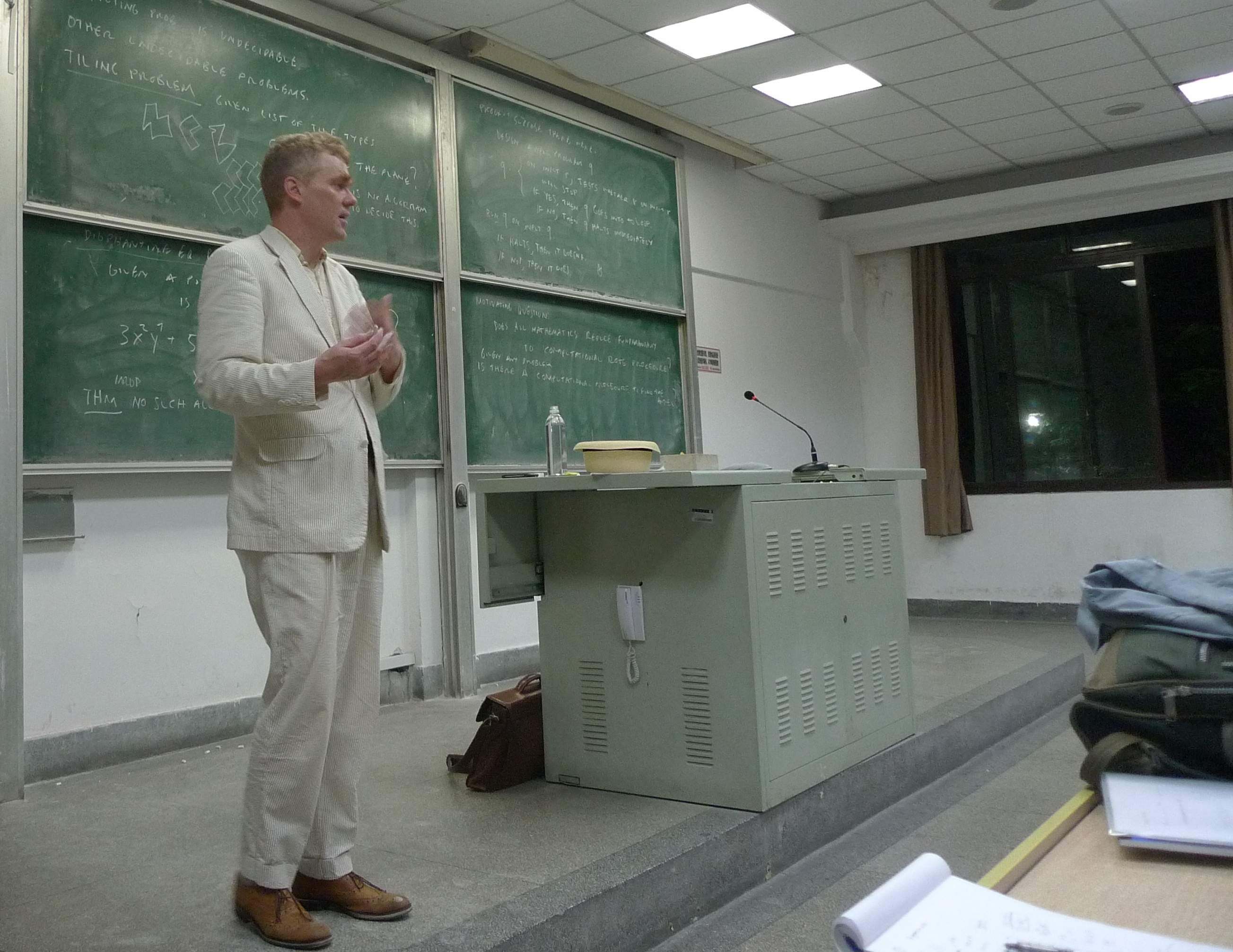
My recent talk, Playful Paradox with large numbers, infinity and logic, was a romp through various paradoxical topics in mathematics and logic for an audience of about 150 mathematics and philosophy undergraduate students at Fudan University in Shanghai, and since Fudan is reportedly a top-three university in China, you can expect that the audience was sharp.

For a bit of fun, and in keeping with the theme, we decided to hold a Largest-Number Contest: what is the largest number that one can describe on an ordinary index card?

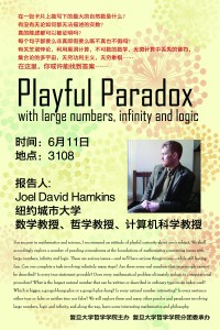
My host Ruizhi Yang made and distributed announcement flyers for the contest a week before the talk, with a poster of the talk on one side, and a description of the contest rules on the other, and including a small card to be used for submissions. The rules were as follows:

A submission entry consists of the description of a positive integer written on an ordinary index card, using common mathematical operations and notation or English words and phrases.
Write legibly, and use at most 100 symbols from the ordinary ASCII character set. Bring your submission to the talk.
Descriptions that fail to describe a number are disqualified.
The submission with the largest number wins.
The prize will be $1 million USD, divided by the winning number itself, rounded to the nearest cent, plus another small token prize.

Example submissions:

$99999$.

$10*(10*99)+5$

The population of Shanghai at this moment.

The submissions were collected at the beginning of my talk, which I began with a nod to Douglas Hofstadter, who once held a similar contest in his column at Scientific American magazine.

To win, I began, it seemed clear that the submitted number must be very large, and since the prize was to be one million dollars divided by the winning number, then this would mean that the prize should become small. So the goal is just to win, and not necessarily to win any money. The real prize is Pride.

So, what kind of numbers should one submit? Of course, anyone could think to write $99999$, or one million ($10^6$), one billion ($10^9$) or one trillion ($10^{12}$). Perhaps someone would want to write a googol, which is a common name for $10^{100}$. Written in decimal, this is $$10000000000000000000000000000000000000000000000000000000000000000000000000000000000000000000000000000,$$ which is one character too long for the rules, so one should use the more compact formulations. But let’s just write it as googol.

But we can easily describe much larger numbers. A googol plex is the number $10^{\text{googol}}$, written in decimal with a $1$ followed by a googol many $0$s. A googol plex is also describable as $10^{10^{100}}$. An iterated exponential $a^{b^c}$ could be seen as ambiguous, referring either to $(a^b)^c$ or to $a^{(b^c)}$. These are not always the same, and so exponentiation is not an associative operation. But which is bigger? If the aim is to make big numbers, then generally one wants to have as big an exponent as possible, and so $a^{(b^c)}$ will be much larger than $(a^b)^c$, which is just $a^{bc}$, and so we will always associate our exponentials upward. (Nevertheless, the upward associated form is not always larger, which you can see in the case of $2^{1^{100}}$.) In general, we can apply the plex operation to any number, so $x$ plex just means $10^x$.

A googol bang means googol !, or googol factorial, the number obtained by multiplying googol $\cdot$ (googol -1) $\cdots 2\cdot 1$, and in general, $x$ bang means $x!$. Which is bigger, a googol plex or a googol bang? If you think about it, a googol plex is 10 times 10 times 10, and so on, with a googol number of terms. Meanwhile, the factorial googol bang also has a googol terms in it, but most of them (except for 10) are far larger than 10, so it is clear that a googol bang is much larger than a googol plex.

Continuing down this road, how about a googol plex bang, or a googol bang plex? Which of these is larger? Please turn away and think about it for a bit……..Have you got it? I think like this: A googol plex bang has the form $(10^g)!$, which is smaller than $(10^g)^{10^g}$, which is equal to $10^{g10^g}$, and this is smaller than $10^{g!}$ when $g$ is large. So a googol plex bang is smaller than a googol bang plex.

There is an entire hierarchy of such numbers, such as googol bang plex bang bang bang and googol bang bang plex plex plex. Which of these is bigger? Do you have a general algorithm for determining which of two such expressions is larger?

A googol stack is the number

$$10^{10^{10^{\cdot^{\cdot^{10}}}}}{\large\rbrace} \text{ a stack of height googol},$$

where the height of the exponential stack is googol. Similarly, we may speak of $x$ stack for any $x$, and form such expressions as:

googol stack bang plex

googol bang plex stack

googol plex stack bang

Which of these is larger? If you think about it, you will see that the stack operator is far more powerful than bang or plex, and so we want to apply it to the biggest possible argument. So the second number is largest, and then the third and then the first, simply because the stack operator will overrule the other effects. Let us call this hierarchy, of all expressions formed by starting with googol and then appending any number of plex, bang or stack operators, as the googol plex bang stack hierarchy.

Question. Is there a feasible computational procedure to determine, of any two expressions in the googol stack bang plex hierarchy, which is larger?

This is an open question in the general case. I had asked this question at math.stackexchange, Help me put these enormous numbers in order, and the best currently known (due to user Deedlit) is that we have a simple algorithm that works for all expressions of length at most googol-2, and also works for all expressions having the same number of operators. But this algorithm breaks down for large expressions of much different lengths, since it seems that one must come to know the exact threshold where an enormous iteration of bangs and plexes can ultimately capture a stack. Of course, in principle one can compute these numbers exactly, given sufficient time and space resources, but the point of the question is to have a feasible algorithm, such as one that takes only polynomial time in the length of the input expressions. And a feasible such general algorithm is not known.

The fact that we seem to have difficulty comparing the relative sizes of expressions even in the simple googol plex bang stack hierarchy suggests that we may find it difficult to select a winning entry in the largest-number contest. And indeed, I’ll explain a bit later why there is no computable procedure to determine the winner of arbitrary size largest-number contests.

The numbers we’ve seen so far are actually rather small, so let’s begin to describe some much larger numbers. The most basic operation on natural numbers is the successor operation $a\mapsto a+1$, and one can view addition as repeated succession:

$$a+b=a+\overbrace{1+1+\cdots+1}^{b\text{ times}}.$$

Similarly, multiplication is repeated addition

$$a\cdot b=\overbrace{a+a+\cdots+a}^{b\text{ times}}$$

and exponentiation is repeated multiplication

$$a^b=\overbrace{a\cdot a\cdots a}^{b\text{ times}}.$$

Similarly, stacks are repeated exponentiation. To simplify the expressions, Knuth introduced his uparrow notation, writing $a\uparrow b$ for $a^b$, and then repeating it as

$$a\uparrow\uparrow b=\overbrace{a\uparrow a\uparrow\cdots\uparrow a}^{b\text{ times}}= a^{a^{a^{.^{.^a}}}}{\large\rbrace}{ b\text{ times}}.$$

So googol stack is the same as $10\uparrow\uparrow$ googol. But why stop here, we can just as easily define the triple repeated uparrow

$$a\uparrow\uparrow\uparrow b=\overbrace{a\uparrow\uparrow a\uparrow\uparrow\ \cdots\ \uparrow\uparrow a}^{b\text{ times}}.$$

In this notation, $10\uparrow\uparrow\uparrow$ googol means

$$\overbrace{10^{10^{.^{.^{10}}}}{\large\rbrace}10^{10^{.^{.^{10}}}}{\large\rbrace}10^{10^{.^{.^{10}}}}{\large\rbrace}\cdots\cdots{\large\rbrace} 10^{10^{.^{.^{10}}}}{\large\rbrace}10}^{\text{iterated googol times}},$$

where the number of times the stacking process is iterated is googol. This number is a vast number, whose description $10\uparrow\uparrow\uparrow$ googol fits easily on an index card.

But why stop there? We could of course continue with $10\uparrow\uparrow\uparrow\uparrow$ googol and so on, but I’d rather define

$$10\Uparrow x=10\ \overbrace{\uparrow\uparrow\cdots\uparrow}^{x\text{ times}}\ 10.$$

So that $10\Uparrow$ googol is vaster than anything we’ve mentioned above. But similarly, we will have $10\Uparrow\Uparrow$ googol and so on, leading eventually to a triple uparrow
$$10 \uparrow\hskip-.55em\Uparrow\text{ googol } = 10 \overbrace{\Uparrow\Uparrow\cdots\Uparrow}^{\text{googol iterations}} 10,$$
and so on. These ideas lead ultimately to the main line of the Ackerman function.

So we’ve described some truly vast numbers. But what is the winning entry? After all, there are only finitely many possible things to write on an index card in accordance with the limitation on the number of symbols. Many of these possible entries do not actually describe a number–perhaps someone might submit a piece of poetry or confess their secret love–but nevertheless among the entries that do describe numbers, there are only finitely many. Thus, it would seem that there must be a largest one. Thus, since the rules expressly allow descriptions of numbers in English, it would seem that we have found our winning entry:

The largest number describable on an index card according to the rules of this contest

which uses exactly 86 symbols. We seem to have argued that this expression describes a particular number, and accords with the rules, so we conclude that this is indeed provably the winning entry.

But wait a minute! If the expression above describes a number, then it would seem that the following expression also describes a number:

The largest number describable on an index card according to the rules of this contest, plus one

which uses 96 symbols. And this number would seem to be larger, by exactly one, of the number which we had previously argued must be the largest number that is possible to describe on an index card. Indeed, how are we able to write this description at all? We seem to have described a number, while following certain rules, that is strictly larger than any number which it is possible to describe while following those rules. Contradiction! This conundrum is known as Berry’s paradox, the paradox of “the smallest positive integer not definable in under eleven words.”

Thus, we can see that this formulation of the largest-number contest is really about the Berry paradox, which I shall leave you to ponder further on your own.

I concluded this part of my talk by discussing the fact that even when one doesn’t allow natural language descriptions, but stays close to a formal language, such as the formal language of arithmetic, then the contest ultimately wades into some difficult waters of mathematical logic. It is a mathematical theorem that there is no computable procedure that will correctly determine which of two descriptions, expressed in that formal language, describes the larger natural number. For example, even if we allow descriptions of the form, “the size of the smallest integer solution to this integer polynomial equation $p(x_1,\ldots,x_k)=0$,” where $p$ is provided as a specific integer polynomial in several variables. The reason is that the halting problem of computability theory is undecidable, and it is reducible to the problem of determining whether such a polynomial equation has a solution, and when it does, the size of the smallest solution is related to the halting time of the given instance of the halting problem. Worse, the independence phenomenon shows that not only is the comparison problem undecidable, but actually there can be specific instances of descriptions of numbers in these formal languages, such that both definitely describe a specific number, but the question of which of the two numbers described is larger is simply independent of our axioms, whatever they may be. That is, the question of whether one description describes a larger number than another or not may simply be neither provable nor refutable in whatever axiomatic system we have chosen to work in, no matter how strong. In such a case, I would find it to be at least a debatable philosophical question whether there is indeed a fact of the matter about whether one of the numbers is larger than the other or not. (See my explanation here). It is my further considered belief that every largest-number contest, taken seriously, unless severely limited in the scope of the descriptions that entries may employ, will founder on precisely this kind of issue.

For further reading on this topic, there are a number of online resources:

Googol plex bang stack hierarchy | Largest number contest on MathOverflow

Scott Aaronson on Big Numbers (related: succinctly naming big numbers)

Meanwhile, lets return to our actual contest, for which we collected a number of interesting submissions, on which I’ll comment below. Several students had appreciated the connection between the contest and Berry’s paradox.

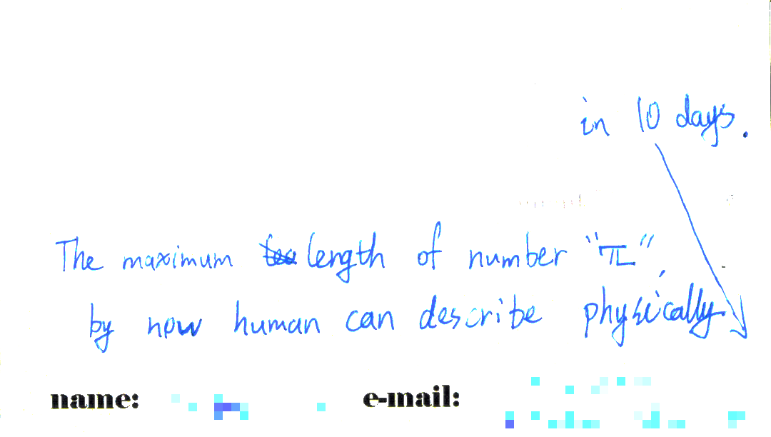
Your number is quite large, since we can surely describe an enormous number of digits of $\pi$. Researchers have announced, for example, that they have now found 10 trillion digits of $\pi$. If by “describe physically” you meant that we should say the digits aloud, however, then supposing that we speak very quickly and say five digits per second (which is quite a lot if sustained for any length of time), then one person would be able to pronounce a little over 4 million digits this way in 10 days. If all humanity were to speak digits in parallel, then we could rise up to the order of $10^{16}$ digits in ten days. This is a big number indeed, although not nearly as big as a googol or many of the other numbers we have discussed.

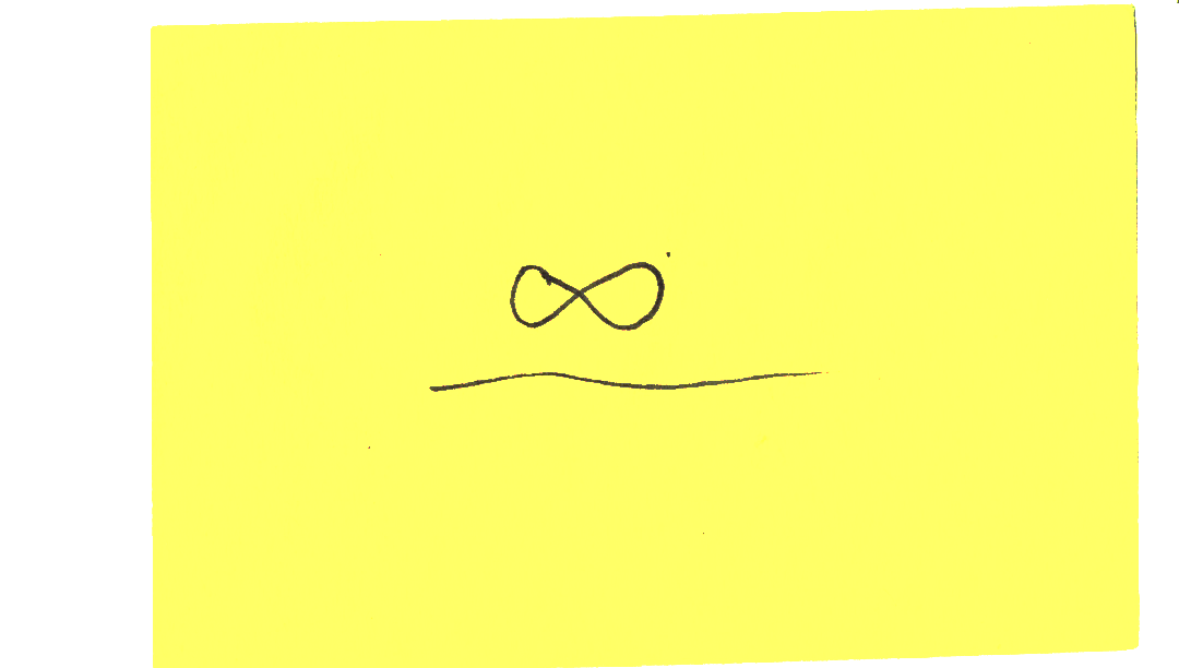
Surely $\infty$ is a large number, but it is not ordinarily considered to be a positive integer or a natural number. And so I think that your submission does not accord with the rules.

This is charming, and I’m sure that your girlfriend will be very happy to see this. Depending on the units we use to measure your affection, I find it very likely that this number is extremely large indeed, and perhaps you win the contest. (But in order to stay within the rules, we should pick the units so that your affection comes out exactly as a positive integer; in particular, if your affection is actually infinite, as you seem to indicate, then I am afraid that you would be disqualified.) One concern that I have, however, about your delightful entry—please correct me if I am wrong—is this: did you write at first about your affection for your “girlfriends” (plural), and then cross out the extra “s” in order to refer to only one girlfriend? And when you refer to your “girlfriend(s), which values at least $\omega$,” do you mean to say that your affection for each girlfriend separately has value $\omega$, or are you instead saying that you have affection for $\omega$ many girlfriends? I’m not exactly sure. But either interpretation would surely lead to a large number, and it does seem quite reasonable that one might indeed have more affection, if one had many girlfriends rather than only one! I suppose we could accept this entry as a separate submission about your affection, one value for each girlfriend separately, but perhaps it may be best to combine all your affection together, and consider this as one entry. In any case, I am sure that you have plenty of affection.

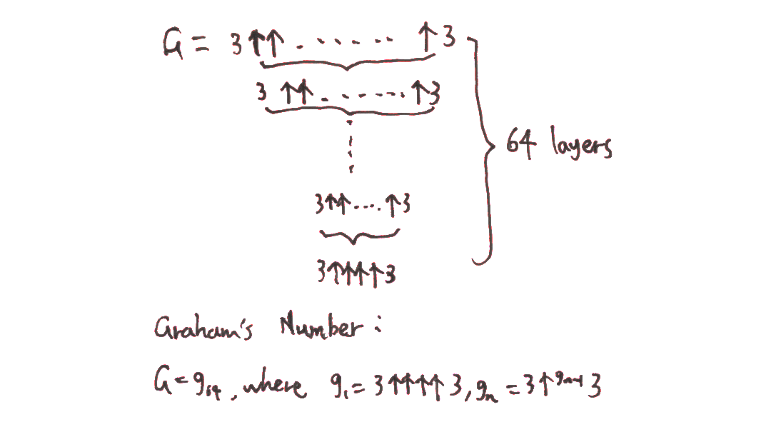
You’ve submitted Graham’s number, an extremely large number that is also popularly known as the largest definite number ever to be used in a published mathematical proof. This number is certainly in the upper vicinity of the numbers we discussed above, obtained by iterating the Knuth uparrow. It is much larger than anything we can easily write in the googol plex bang stack hierarchy. This is essentially in line with iterating the $\Uparrow$ operator $64$ times, using base $3$. This number is extremely large, and I find it to be the largest number submitted by means of a definite description whose numerical value does not depend on which other numbers have been submitted to the contest. Meanwhile, we discussed some even larger numbers above, such as the triple uparrow $10 \uparrow\hskip-.55em\Uparrow$ googol.

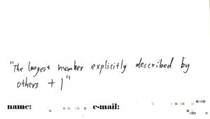
Your clever submission shows that you realize that it isn’t necessary to actually mention the largest possible number to describe, as we discussed in Berry’s paradox above, but it suffices rather to exceed only the largest actually occurring numbers that are described by others in the contest. What are we to do, however, when two people have this same clever idea? If either of them succeeds in describing a number, then it would seem that they both must succeed, but in this case, they must both have described numbers larger than the other. This is the same contradiction at the heart of Berry’s paradox. Another risky feature of this entry is that it presumes that some numbers were in fact described by others. How are we to interpret it if all other submissions are disqualified?

Your description has the very nice feature that it avoids the self-reference needed in the previous description to refer to all the “other” entries (that is, all the entries that are not “this” one). It avoids the self-reference by speaking of “second-largest” entry, which of course will have to be the largest of the other entries, since this entry is to be one larger. Although it avoids self-reference, nevertheless this description is what would be called impredicative, because it quantifies over a class of objects (the collected entries) of which it is itself a member. Once one interprets things as you seem to intend, however, this entry appears to amount to essentially the same description as the previous entry. Thus, the problematic and paradoxical situation has now actually occurred, making it problematic to conclude that either of these entries has succeeded in describing a definite number. So how are we to resolve it?

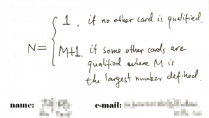
Your description is very clever, trying to have it both ways. Of course, every participant in the contest wants to win, but you also to win with a very low winning number, so that you can maximize the prize payout. With this submission, of course you hope that all other submissions might be disqualified, in which case you will win with the number 1, achieving the million dollar payout! In the case of our actual contest, however, there are other cards that are qualified, such as the Graham’s number submission, and so your submission seems to be in case 2, making it similar in effect to the previous submission. Like the previous two entries, this card is problematic when two or more players submit the same description. And indeed, even with the other descriptions submitted above, we are already placed into the paradoxical situation that if this card describes a number in its case 2, then it will be larger than some numbers that are larger than it.

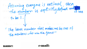
Your submission is very ambitious, attempting both to win and to win the most money. (I take the description as the lower part of this card, and the upper note is a remark about it.) You seem to realize that there will be ties in the game, with multiple people submitting a winning entry. And indeed, if everyone had submitted this entry, then the winning number would indeed seem to be 1, which is the smallest number that would make them all be one of the members who win the game, so the million dollars would be split amongst that group. Some clumsy person, however, might submit a googol plex bang, however, which would bump up the value of this card to that same value, which although still winning, would win much less money. Your line of reasoning about rationality is very similar to the concept of superrationality defended by Douglas Hofstadter in the context of the prisoner’s dilemma. Perhaps one might also be tempted to say something like:

the smallest number that makes me win, with the largest possible prize payout to me.

with the idea that you’d get a bigger prize solely for yourself if you avoided a tie situation by adding one more, so as to get the whole prize for yourself. But if this reasoning is correct, then one would seem to land again in the clutches of the Berry paradox.

To my readers: please make your submissions or comments below!

More math for six-year-olds: Win at Nim!

Posted on May 20, 2013 by Joel David Hamkins

The latest installment of math for six-year-olds…

Win at Nim!
Fold up the bottom flap to prevent parents from learning the super-secret strategy.

This morning once again I went into my daughter’s first-grade classroom, full of inquisitive six-and-seven-year-old girls, and made a mathematical presentation on the game of Nim.

Win at Nim!

The game of Nim, I explained, begins with one player setting up a number of stacks of blocks,while the opponent chooses whether to go first or second. Taking turns, each player removes one or more blocks from a stack of their choosing. (It is fine to take a whole stack on your turn.) The player who takes the last block wins.

We demonstrated the game by playing a number of exhibition rounds, and then the girls divided into pairs to play each other and also me. They were surprised that I was able to win against them every single time. In explanation, I told them that this was because in the game of Nim, there is a super-secret mathematical strategy! Did they want to learn? Yes! I took as my goal that they would all learn the Nim strategy, so that they could go home and confound their parents by beating them again and again at the game.

Since this was a first-grade class, we concentrated at first on games with stacks of heights 1, 2 and 3 only, a special case of the game which can still challenge adults, but for which six-year-olds can easily learn the winning strategy.

Two balanced stacks

After gaining some familiarity with the game by playing several rounds amongst each other, we gathered again for the secret strategy session. We began by thinking about the case of a game of Nim with only two stacks. They had noticed that sometimes when I played them, I had made copying moves; and indeed I had purposely said, “I copy you,” each time this had occurred. The copying idea is surely appealing when there are only two stacks. After some discussion, the girls realized that with just two stacks, if one played so as to equalize them, then one would always be able to copy the opponent’s move. In particular, this copying strategy would ensure that one had a move to make whenever the opponent did, and so one would win the game.

A balanced position

In short order, the girls also realized that if one had any number of pairs of such balanced stacks—so that every stack had a partner—then the whole position was also winning (for one to give to the other player), since one could copy a move on any stack by making the corresponding move on the partner stack. Thus, we deduced that if we could match up stacks of equal height in pairs, then we had a winning strategy, the strategy to copy any move on a partner stack.

In particular, this balancing idea provides a complete winning strategy in the case of Nim games for which all stacks have height one or two. One should play so as to give a balanced position to one’s opponent, namely, a position with an even number of stacks of height one and an even number of stacks of height two. Any unbalanced position can always be balanced in this way, and any move on a balanced position will unbalance it.

1+2+3 counts as balanced

To handle positions with stacks of height three, the super-secret trick is that one can balance a stack of height three either with another stack of height three, of course, but also with two stacks: one of height one and one of height two. Thus, one should regard a stack of height three as consisting of two sub-stacks, one of height one and one of height two, for the purposes of balancing. Thus, the Nim position 1+2+3 counts as balanced, since the 3 counts as 2+1, which balances the other stacks. The 1+2+3 position has two stacks of height two and two of height one, when one regards the stack of height three as having a substack of height two and a substack of height one.

In this way, one arrives at a complete winning strategy for Nim positions involving stacks of height at most three, and furthermore, this is a strategy that can be mastered by first-graders. The strategy is to strive to balance the position. If you always give your opponent a balanced position, then you will win! Faced with an unbalanced position, you can always find a balancing move, and any move on an balanced position will unbalance it. If the game is just starting, and you are deciding whether to go first or second, you should determine whether it is balanced yet or not. If it unbalanced, then you should go first and make the balancing move; if it is already balanced, then you should go second and adopt the copying strategy, in which you re-balance the position with each move.

More advanced players will want to consider Nim positions with taller stacks than three, and we talked about this a little in the classroom. Some of the girls realized that the copying strategy and the idea of balanced positions still worked with taller stacks. One can balanced stacks of height four against other stacks of height four, and so one, but the trick for these taller stacks is that one may balance 5 with 4+1; balance 6 with 4+2; and 7 with 4+2+1. Mathematicians will recognize here the powers of two.

To teach the strategy to children, it is a great opportunity to talk about the powers of two. Any child knows how to count 1, 2, 3, 4 and so on, and most can count by twos 2, 4, 6, 8, 10, …; by fives 5, 10, 15, 20, …; by tens, by threes; by sevens; and so on. , The powers of two are the numbers 1, 2, 4, 8, 16, 32, 64, 128, and so on, doubling each time. Climbing this exponential growth, children are often amazed at how quickly one reaches very large numbers:

One plus one is two;

two plus two is four;

four plus four is eight;

eight plus eight is sixteen;

sixteen plus sixteen is thirty-two;

thirty-two plus thirty-two is sixty-four;

sixty-four plus sixty-four is one hundred twenty-eight.

For Nim, we don’t in practice need such big powers of two, since one doesn’t usually encounter stacks of height eight or larger, and usually just 1s, 2s and 4s suffice. The relevant fact for us here is that every natural number is uniquely expressible as a sum of distinct powers of two, which of course is just another way of talking about binary representation of a number in base two. We regard a Nim stack as consisting of its power-of-two substacks. Thus, a stack of height 3 counts as 2+1; a stack of height 5 counts as 4+1; a stack of height 6 counts as 4+2; and a stack of height 7 counts as 4+2+1.

Ultimately, the winning general strategy for Nim is always to play so as to balance the position, where one regards every stack as being composed of its power-of-two sub-stacks, and a position counts as balanced when these stacks and sub-stacks can be matched up in pairs. This is a winning strategy, since every unbalanced position can be balanced, and any move on a balanced position will unbalance it. To balance an unbalanced stack, play on any stack containing the largest size unbalanced power of two substack, and reduce it so as to balance the parity of all the stacks. If one thinks about it, at bottom what we are doing is ensuring that if we represent the stack heights in their binary representation, then we should play so as to ensure that the position has a even number of one digits in each place.

Math for six-year-olds

Posted on February 4, 2013 by Joel David Hamkins

Today I went into my daughter’s first-grade classroom, full of six-year-old girls, and gave a presentation about Möbius bands.

We cut strips of paper and at first curled them into simple bands, cylinders, which we proved had two sides by coloring them one color on the outside and another color on the inside. Next, we cut strips and curled them around, but added a twist, to make a true Möbius band.

A Möbius band

These, of course, have only one side, a fact that the children proved by coloring it one color all the way around. And we observed that a Möbius band has only one edge.

A Möbius-like band, with two twists

We explored what happens with two twists, or more twists, and also what happens when you cut a Möbius band down the center, all the way around.

Möbius band cut down the center

It is very interesting to cut a Möbius band on a line that is one-third of the way in from an edge, all the way around. What happens? Make your prediction before unraveling the pieces–how many pieces will there be? Will they be all the same size? How many twists will they have?

Overall, the whole presentation was a lot of fun. The girls were extremely curious about everything, and experimented with additional twists and additional ways of cutting. It seemed to be just the right amount of mathematical thinking, cutting and coloring for a first-grade class. To be sure, without prompting the girls made various Möbius earrings, headbands and bracelets, which I had to admit were fairly cool. One girl asked, “is this really mathematics?”

It seems I may be back in the first-grade classroom this spring, and I have in mind to teach them all how to beat their parents at Nim.

The differential operator $\frac{d}{dx}$ binds variables

Posted on December 5, 2012 by Joel David Hamkins

Recently the question If $\frac{d}{dx}$ is an operator, on what does it operate? was asked on mathoverflow. It seems that some users there objected to the question, apparently interpreting it as an elementary inquiry about what kind of thing is a differential operator, and on this interpretation, I would agree that the question would not be right for mathoverflow. And so the question was closed down (and then reopened, and then closed again….sigh). (Update 12/6/12: it was opened again,and so I’ve now posted my answer over there.)

Meanwhile, I find the question to be more interesting than that, and I believe that the OP intends the question in the way I am interpreting it, namely, as a logic question, a question about the nature of mathematical reference, about the connection between our mathematical symbols and the abstract mathematical objects to which we take them to refer. And specifically, about the curious form of variable binding that expressions involving $dx$ seem to involve. So let me write here the answer that I had intended to post on mathoverflow:

————————-

To my way of thinking, this is a serious question, and I am not really satisfied by the other answers and comments, which seem to answer a different question than the one that I find interesting here.

The problem is this. We want to regard $\frac{d}{dx}$ as an operator in the abstract senses mentioned by several of the other comments and answers. In the most elementary situation, it operates on a functions of a single real variable, returning another such function, the derivative. And the same for $\frac{d}{dt}$.

The problem is that, described this way, the operators $\frac{d}{dx}$ and $\frac{d}{dt}$ seem to be the same operator, namely, the operator that takes a function to its derivative, but nevertheless we cannot seem freely to substitute these symbols for
one another in formal expressions. For example, if an instructor were to write $\frac{d}{dt}x^3=3x^2$, a student might object, “don’t you mean $\frac{d}{dx}$?” and the instructor would likely reply, “Oh, yes, excuse me, I meant $\frac{d}{dx}x^3=3x^2$. The other expression would have a different meaning.”

But if they are the same operator, why don’t the two expressions have the same meaning? Why can’t we freely substitute different names for this operator and get the same result? What is going on with the logic of reference here?

The situation is that the operator $\frac{d}{dx}$ seems to make sense only when applied to functions whose independent variable is described by the symbol “x”. But this collides with the idea that what the function is at bottom has nothing to do with the way we represent it, with the particular symbols that we might use to express which function is meant. That is, the function is the abstract object (whether interpreted in set theory or category theory or whatever foundational theory), and is not connected in any intimate way with the symbol “$x$”. Surely the functions $x\mapsto x^3$ and $t\mapsto t^3$, with the same domain and codomain, are simply different ways of describing exactly the same function. So why can’t we seem to substitute them for one another in the formal expressions?

The answer is that the syntactic use of $\frac{d}{dx}$ in a formal expression involves a kind of binding of the variable $x$.

Consider the issue of collision of bound variables in first order logic: if $\varphi(x)$ is the assertion that $x$ is not maximal with respect to $\lt$, expressed by $\exists y\ x\lt y$, then $\varphi(y)$, the assertion that $y$ is not maximal, is not correctly described as the assertion $\exists y\ y\lt y$, which is what would be obtained by simply replacing the occurrence of $x$ in $\varphi(x)$ with the symbol $y$. For the intended meaning, we cannot simply syntactically replace the occurrence of $x$ with the symbol $y$, if that occurrence of $x$ falls under the scope of a quantifier.

Similarly, although the functions $x\mapsto x^3$ and $t\mapsto t^3$ are equal as functions of a real variable, we cannot simply syntactically substitute the expression $x^3$ for $t^3$ in $\frac{d}{dt}t^3$ to get $\frac{d}{dt}x^3$. One might even take the latter as a kind of ill-formed expression, without further explanation of how $x^3$ is to be taken as a function of $t$.

So the expression $\frac{d}{dx}$ causes a binding of the variable $x$, much like a quantifier might, and this prevents free substitution in just the way that collision does. But the case here is not quite the same as the way $x$ is a bound variable in $\int_0^1 x^3\ dx$, since $x$ remains free in $\frac{d}{dx}x^3$, but we would say that $\int_0^1 x^3\ dx$ has the same meaning as $\int_0^1 y^3\ dy$.

Of course, the issue evaporates if one uses a notation, such as the $\lambda$-calculus, which insists that one be completely explicit about which syntactic variables are to be regarded as the independent variables of a functional term, as in $\lambda x.x^3$, which means the function of the variable $x$ with value $x^3$. And this is how I take several of the other answers to the question, namely, that the use of the operator $\frac{d}{dx}$ indicates that one has previously indicated which of the arguments of the given function is to be regarded as $x$, and it is with respect to this argument that one is differentiating. In practice, this is almost always clear without much remark. For example, our use of $\frac{\partial}{\partial x}$ and $\frac{\partial}{\partial y}$ seems to manage very well in complex situations, sometimes with dozens of variables running around, without adopting the onerous formalism of the $\lambda$-calculus, even if that formalism is what these solutions are essentially really about.

Meanwhile, it is easy to make examples where one must be very specific about which variables are the independent variable and which are not, as Todd mentions in his comment to David’s answer. For example, cases like

$$\frac{d}{dx}\int_0^x(t^2+x^3)dt\qquad
\frac{d}{dt}\int_t^x(t^2+x^3)dt$$

are surely clarified for students by a discussion of the usage of variables in formal expressions and more specifically the issue of bound and free variables.

Hello world!

Posted on September 22, 2011 by Joel David Hamkins

I am pleased to join Booles’ Rings, and looking forward to the goings-on here! Sam Coskey has been an enormous help in getting me set up here, for which I am very thankful. I will be adding more information in the near future.

Joel David Hamkins

mathematics and philosophy of the infinite

Category Archives: Exposition

A common forcing extension obtained via different forcing notions

Local properties in set theory

Math for seven-year-olds: graph coloring, chromatic numbers, and Eulerian paths and circuits

Uniform $({\lt}\theta)$-supercompactness is equivalent to a coherent system of normal fine measures

Large cardinal indestructibility: two slick new proofs of prior results

Kelley-Morse set theory implies Con(ZFC) and much more

Approximation and cover properties propagate upward

Largest-number contest: what is the largest number that you can describe on an index card?

More math for six-year-olds: Win at Nim!

Math for six-year-olds

The differential operator $\frac{d}{dx}$ binds variables

Hello world!

Share:

Share:

Share:

Share:

Share:

Share:

Share:

Share:

Share:

Share:

Share:

Share: