Here is an interesting game I heard a few days ago from one of my undergraduate students; I’m not sure of the provenance.
The game is played with stones on a grid, which extends indefinitely upward and to the right, like the lattice $\mathbb{N}\times\mathbb{N}$. The game begins with three stones in the squares nearest the origin at the lower left. The goal of the game is to vacate all stones from those three squares. At any stage of the game, you may remove a stone and replace it with two stones, one in the square above and one in the square to the right, provided that both of those squares are currently unoccupied.
For example, here is a sample play.

Question. Can you play so as completely to vacate the yellow corner region?
One needs only to move the other stones out of the way so that the corner stones have room to move out. Can you do it? It isn’t so easy, but I encourage you to try.
Here is an online version of the game that I coded up quickly in Scratch: Escape!
My student mentioned the problem to me and some other students in my office on the day of the final exam, and we puzzled over it, but then it was time for the final exam. So I had a chance to think about it while giving the exam and came upon a solution. I’ll post my answer later on, but I’d like to give everyone a chance to think about it first.
Solution. Here is the solution I hit upon, and it seems that many others also found this solution. The main idea is to assign an invariant to the game positions. Let us assign weights to the squares in the lattice according to the following pattern. We give the corner square weight $1/2$, the next diagonal of squares $1/4$ each, and then $1/8$, and so on throughout the whole playing board. Every square should get a corresponding weight according to the indicated pattern.
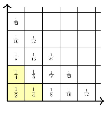
The weights are specifically arranged so that making a move in the game preserves the total weight of the occupied squares. That is, the total weight of the occupied squares is invariant as play proceeds, because moving a stone with weight $1/2^k$ will create two stones of weight $1/2^{k+1}$, which adds up to the same. Since the original three stones have total weight $\frac 12+\frac14+\frac14=1$, it follows that the total weight remains $1$ after every move in the game.
Meanwhile, let us consider the total weight of all the squares on the board. If you consider the bottom row only, the weights add to $\frac12+\frac14+\frac18+\cdots$, which is the geometric series with sum $1$. The next row has total weight $\frac14+\frac18+\frac1{16}+\cdots$, which adds to $1/2$. And the next adds to $1/4$ and so on. So the total weight of all the squares on the board is $1+\frac12+\frac14+\cdots$, which is $2$. Since we have $k$ stones with weight $1/2^k$, another way to think about it is that we are essentially establishing the sum $\sum_k\frac k{2^k}=2$.
The subtle conclusion is that after any finite number of moves, only finitely many of those other squares are occupied, and so some of them remain empty. So after only finitely many moves, the total weight of the occupied squares off of the original L-shape is strictly less than $1$. Since the total weight of all the occupied squares is exactly $1$, this means that the L-shape has not been vacated.
So it is impossible to vacate the original L-shape in finitely many moves. $\Box$
Suppose that we relax the one-stone-per-square requirement, and allow you to stack several stones on a single square, provided that you eventually unstack them. In other words, can you play the stacked version of the game, so as to vacate the original three squares, provided that all the piled-up stones eventually are unstacked?
No, it is impossible! And the proof is the same invariant-weight argument as above. The invariance argument does not rely on the one-stone-per-square rule during play, since it is still an invariant if one multiplies the weight of a square by the number of stones resting upon it. So we cannot transform the original stones, with total weight $1$, to any finite number of stones on the rest of the board (with one stone per square in the final position), since those other squares do not have sufficient weight to add up to $1$, even if we allow them to be stacked during intermediate stages of play.
Meanwhile, let us consider playing the game on a finite $n\times n$ board, with the rule modified so that stones that would be created in row or column $n+1$ in the infinite game simply do not materialize in the $n\times n$ game. This breaks the proof, since the weight is no longer an invariant for moves on the outer edges. Furthermore, one can win this version of the game. It is easy to see that one can systematically vacate all stones on the upper and outer edges, simply by moving any of them that is available, pushing the remaining stones closer to the outer corner and into oblivion. Similarly, one can vacate the penultimate outer edges, by doing the same thing, which will push stones into the outer edges, which can then be vacated. By reverse induction from the outer edges in, one can vacate every single row and column. Thus, for play on this finite board with the modified rule on the outer edges, one can vacate the entire $n\times n$ board!
Indeed, in the finite $n\times n$ version of the game, there is no way to lose! If one simply continues making legal moves as long as this is possible, then the board will eventually be completely vacated. To see this, notice first that if there are stones on the board, then there is at least one legal move. Suppose that we can make an infinite sequence of legal moves on the $n\times n$ board. Since there are only finitely many squares, some of the squares must have been moved-upon infinitely often. If you consider such a square closest to the origin (or of minimal weight in the scheme of weights above), then since the lower squares are activated only finitely often, it is clear that eventually the given square will replenished for the last time. So it cannot have been activated infinitely often. (Alternatively, argue by induction on squares from the lower left that they are moved-upon at most finitely often.) Indeed, I claim that the number of steps to win, vacating the $n\times n$ board, does not depend on the order of play. One can see this by thinking about the path of a given stone and its clones through the board, ignoring the requirement that a given square carries only one stone. That is, let us make all the moves in parallel time. Since there is no interaction between the stones that would otherwise interfere, it is clear that the number of stones appearing on a given square in total is independent of the order of play. A tenacious person could calculate the sum exactly: each square is becomes occupied by a number of stones that is equal to the number of grid paths to it from one of the original three stones, and one could use this sum to calculate the total length of play on the $n\times n$ board.
 or CC BY-SA 3.0 (http://creativecommons.org/licenses/by-sa/3.0)], via Wikimedia Commons")

 [GFDL (http://www.gnu.org/copyleft/fdl.html), CC-BY-SA-3.0 (http://creativecommons.org/licenses/by-sa/3.0/) or CC BY-SA 2.5-2.0-1.0 (http://creativecommons.org/licenses/by-sa/2.5-2.0-1.0)], via Wikimedia Commons")
_croped.jpg)